1. Introduction
he euro greatly depreciated against the dollar during the period 1995-2001. This decline has often been associated with relative productivity changes in the United States and the euro area over this time period. During this time period in particular, average labor productivity accelerated in the United States, while it decelerated in the euro area. Economic theory suggests that the equilibrium real exchange rate will appreciate after an actual or expected shock in average labor productivity in the traded goods sector. Such an equilibrium appreciation may be influenced in the medium term by demand side effects. Thus, productivity increases raise expected income, which leads to an increased demand for goods. However, the price of goods in the traded sector is determined more by international competition. By contrast, in the nontraded sector, where industries are not subject to the same competition, goods prices tend to vary widely and independently across countries.
The work of Harrod (1933), Balassa (1964), and Samuelson (1964) show that productivity growth will lead to a real exchange rate appreciation only if it is concentrated in the traded goods sector of an economy. Productivity growth that has been equally strong in the traded and non-traded sectors will have no effect on the real exchange rate.
Author : Economics Department Nova Southeastern University. H. Wayne Huizenga School of Business and Entrepreneurship. 3301 College Ave. Fort Lauderdale, Florida USA. E-mail : [email protected] From the first to the second half of the 1990's, average productivity accelerated in the United States, while it decelerated in the euro area. This relationship has stimulated a discussion on the relationship between productivity and appreciation of the dollar during this time period. Also, of equal importance is the depreciation of the dollar during the early part of the 2000's (United States productivity increased slowly while the euro area productivity increased more rapidly). Bailey and Wells (2001), for instance, argue that a structured improvement in US productivity increased the rate of return on capital and triggered substantial capital flows in the United States, which might explain in part the appreciation of the US dollar during the early part of the 2000's. Tille and Stoffels (2001) confirm empirically that developments in relative labor productivity can account for part of the change in the external value of the US dollar over the last 3 decades. Alquist and Chinn (2002) argue in favor of a robust correlation between the euro area United States labor productivity differential and the dollar/euro exchange rate. This would explain the largest part of the euro's decline during the latter part of the 1990's.
This paper presents the argument that the euro's persistent weakness in the 1995-2001 period and its strength during the 2001-2007 period can be partly explained by taking into consideration productivity differentials. In particular, the study analyses in detail the impact of relative productivity developments in the United States and the euro area on the dollar/euro exchange rate.
The paper is organized with the first part being the introduction. The next section explains the relationship between productivity advances and the real exchange rate from a theoretical perspective along with the data gathering process. Section 3 deals with the estimation, the structural VECM and impulse response analysis. Section 4 deals with tests for nonnormality and forecast error variance decomposition. Section 5 deals with a discussion of results.
2. II.
3. The Real Exchange Rate and Productivity Developments
The theoretical relationships that link fundamentals to the real exchange rate in the long-run Year This paper analyses the impact of relative productivity developments in the United States and the euro area on the dollar/euro exchange rate. This paper then provides evidence on the long-run relationship between the real dollar/euro exchange rate and productivity measures with and without the oil prices and government spending variables. Importantly, to the extend that traders in foreign exchange markets respond to the available productivity data stresses the importance of reliable models. center around the Balassa-Samuelson model, portfolio balance considerations as well as the uncovered (real) interest rate parity condition. This study will focus on the role of productivity differentials in the determination of the dollar/euro exchange rate.
According to the Balassa-Samuelson framework, the distribution of productivity gains between countries and across tradable and non-tradable goods sectors in each country is important for assessing the impact of productivity advances on the real exchange rate. The intuition behind the Balassa-Samuelson effect is rather straight-forward. Assuming, for instance of simplicity, that productivity in the traded goods sector increases only in the home country, marginal costs will fall for domestic firms in the traded-goods sector. This leads (under the perfect competition condition) to a rise in wages in the traded goods sector at given prices. If labor is mobile between sectors in the economy, workers shift from the non-traded sector to the traded sector in response to the higher wages. This triggers a wage rise in the non-traded goods sector as well, until wages equalize again across sectors. However, since the increase in wages in the non-traded goods sector is not accompanied by productivity gains, firms need to increase their prices, which do not jeopardize the international price competitiveness of firms in the traded goods sector Harrod (1933), Balassa (1964) and Samuelson (1964).
Tille, Stoffels and Gorbachev (2001) revealed that nearly two-thirds of the appreciation of the dollar was attributable to productivity growth differentials (using the traded and nontraded differentials). However, it is important to note that Engel (1999) found that the relative price of non-traded goods accounts almost entirely for the volatility of US real exchange rates. . Accordingly, there should be a proportional link between relative prices and relative productivity. Labor productivity, however, is also influenced by demand-side factors, though their effect should be of a transitory rather than of a permanent nature.
In particular, as the productivity increases raise future income, and if consumers value current consumption more than future consumption, they will try to smooth their consumption pattern as argued by (Bailey and Wells 2001). This leads to an immediate increased demand for both traded and non-traded goods. The increase in demand for traded goods can be satisfied by running a trade deficit. The increased demand for non-traded goods, however, cannot be satisfied and will lead to an increase in prices of non-traded goods instead. Thus, demand effects lead to a relative price shift and thereby to a real appreciation.
a) The Asymptotically Stationary Process of the Model This section presents evidence in favor of stable long-run relationships between the real dollar/euro exchange rate, the productivity measure, and the other variables. One model specification was estimated for the productivity measure. The sample covers the period from 1985 to 2007. The general model includes all variables discussed above as well as deterministic components.
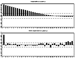
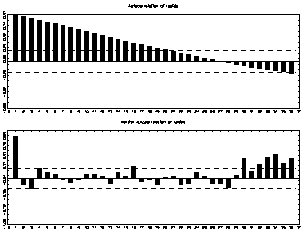
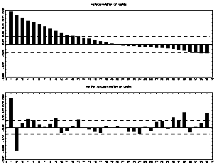
The results of the autocorrelations and partial autocorrelations in figures 1-3 show that the autocorrelations typically die out over time with increasing time as in the GDP, oil prices and US productivity variables. The dashed lines are just +/-2/?T lines; consequently, they give a rough indication of whether the autocorrelation coefficients may be regarded as coming from a process with true autocorrelations equal to zero. A stationary process for which all autocorrelations are zero is called white noise or a white noise process. Clearly, all of the series are not likely to be generated by a white noise process because the autocorrelations reach outside the area between the dashed lines for more than 50% of the time series. On the other hand, all coefficients at higher lags are clearly between the lines. Hence, the underlying autocorrelation function may be in line with a stationary data gathering process. The partial correlations convey basically the same information on the properties of the time series. Gov_Spending Lutkepohl (2004) states that autocorrelations and partial autocorrelations provide useful information on specific properties of a data gathering process other than stationarity. Consistency and asymptotic normality of the maximum likelihood estimators are required for the asymptotic statistical theory behind the tests to be valid. The results of these tests are shown in the appendix (table 6). They consist of an LM test of no error autocorrelation, an LM-type test of no additive nonlinearity, and another LM-type test of parameter constancy. Bartlett (1950) and Parzen (1961) have proposed spectral windows to ensure consistent estimators.
The autocorrelations of a stationary stochastic process may be summarized compactly in the spectral density function. It is defined as
F y (?) = (2?) -1 ? y/? -i?j = (2?) -1 [yo 2 ? yj cos(?j)](1)Where I = ?-1 is the imaginary unit, ??{-?, ?}is the frequency, that is, the number of cycles in a unit of time measured in radians, and the yj's are the autocovariances of y t as before. It can be shown that
Yj = ? Fy (?)d? (2)Thus, the autocovariances can be recovered from the spectral density function integral as follows:
Yo = ? 2 y (?)d?(3)Graph 1 shows the log of the smoothed spectral density estimator based on a Bartlett window with window width M r = 20.
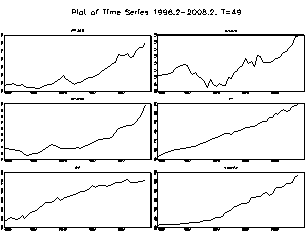
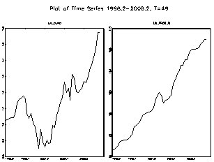
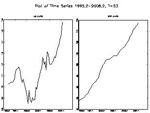
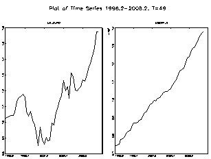
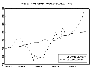
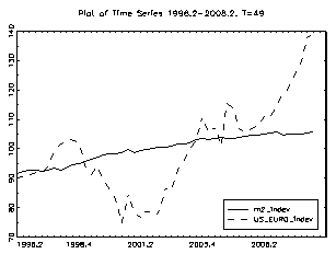
Many economic time series have characteristics incompatible with a stationary data gathering process. However, Lutkepohl (2004) recommends the use of simple transformations to move a series closer to stationarity. A logarithmic transformation may help stabilize the variance. In figure 4 the logarithms of the US productivity, M2, oil prices, US GDP, US/euro exchange rate and government spending are plotted. The logarithm is used as it ensures that larger values remain larger than smaller ones.
The relative size is reduced, however. The series has an upward trend and a distinct seasonal pattern. The series clearly has important characteristics of a stationary series The empirical analysis employs cointegration tests as developed by Johansen (1995). In the present setting, some variables would theoretically be expected to be stationary, but appear to be near-integrated processes empirically.
The presence of the cointegration relationships is tested in a multivariate setting. Table 2 and 3 show the results of the cointegration tests. Over all, the results suggest that it is reasonable to assume a single cointegration relationship between the variables and suggest being viewed as an order of I(1). Significance at the 99%, 95% and 90% levels are noted by ***, ** and * respectively. The S and L critical values are taken from tables computed by Saikkonen and Lutkepohl.
4. c) Data for Variables
For the period prior to 1999, the real dollar/euro exchange rate was computed as a weighted geometric average of the bilateral exchange rates of the euro currencies against the dollar. In addition, the model was estimated controlling for several other variables, which included US productivity, M2, oil prices, government spending and US GDP. As regards the real price of oil, its usefulness for explaining trends in real exchange rates is documented. For example, Amano and Van Norden (1998a and 1998b) found strong evidence of a long-term relationship between the real effective exchange rate of the US dollar and the oil price. As regards government spending, the fiscal balance constitutes one of the key components of national saving. In particular, Frenkel and Mussa (1985) argued that a fiscal tightening causes a permanent increase in the net foreign asset position of a country, and consequently, an appreciation of its equilibrium exchange rate in the long term. This will occur provided that the fiscal consolidation is considered to have a long-run affect. This study shows how much of the decline of the euro against the US dollar during the 1995-2001 period can be attributed to relative changes in productivity in the United States and the euro area.
While the estimation covers the period 1985-2007, the following analysis concentrates on two distinct periods.
Period 1 (1995-2001) covers the US dollar appreciation against the euro.
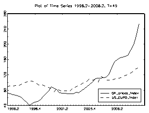
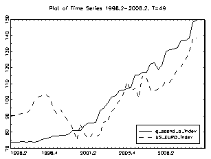
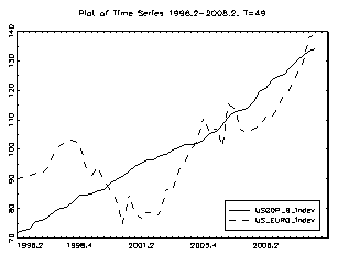
Moreover, it encompasses the period during which the productivity revival in the United States has taken place. Over this period, the dollar appreciated by almost 41%.against the euro area currency. During the first three years (1998-2001) of the euro, it depreciated by almost 30% against the US dollar. Figure 5 shows the impact of a change in relative productivity developments over these periods on the equilibrium real exchange rate. The contribution of the relative developments in productivity on the explanation of the depreciation of the euro against the US dollar since 1995 is significant. However, these developments are far from explaining the entire euro decline. Figures 6 and 7 show the impact of a change in relative US GDP and Euro GDP on the equilibrium dollar/euro real exchange rate.
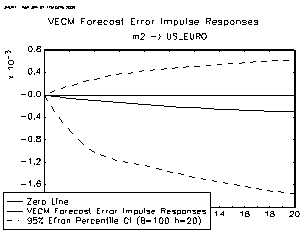
Period 2 (2001-2007) covers the US dollar depreciation against the euro. Figure 8 also shows the impact of a change in relative productivity developments over these periods on the equilibrium real exchange rate. The impact of productivity on the real exchange rate is significant. The contributions of the oil prices, US GDP, M2 and US government spending on the explanation of the volatility of the euro against the US dollar since 1995 are also shown in Figures 9-12. Estimation and The Structural Vecm Lutkepohl (2004) suggests the following basic vector autore gressive and error correction model (neglecting deterministic terns and exogenous variables):
For a set of K times series variables (4)
The VAR model is general enough to accommodate variables with stochastic trends, it is not the most suitable type of model if interest centers on the cointegration relations because they do not appear explicitly.
The following VECM form is a more convenient model setup for cointegration analysis:
(5) a) Deterministic Terms Several extensions of the basic model are usually necessary to represent the main characteristics of a data set. It is clear that including deterministic terms, such as an intercept, a linear trend term, or seasonal dummy variables, may be required for a proper representation of the data gathering process. One way to include deterministic terms is simple to add them to the stochastic part, (6) Here ? t is the deterministic part and x t is a stochastic process that may have a VAR or VECM representation.
A VAR representation for y t is as follows:
A VECM (p-1) representation has the form
y t = ? 0 + ? 1 t + y t-1 Ð?" I Î?" y t-1 + . . . Ð?" p-1 Î?" t-p+1 + ? t(8)b) Exogenous Variables Lutkepohl (2004) recommends further generalizations of the model to include further stochastic variables in addition to the deterministic part. A rather general VECM form that includes all these terms is y t = y t-1 + Ð?" I Î?" y t-1 + . . . Ð?" p-1 Î?" t-p+1 + CD t ? zt + ? t (9) where the zt are unmodeled stochastic variables, D t contains all regressors associated with deterministic terms, and C and ? are parameter matrices. The z 's are considered unmodeled because there are no explanatory equations for them in the system. c) Estimation of VECM's Under Gaussian assumptions estimators are ML estimators conditioned on the presample values (Johansen 1988). They are consistent and jointly asymptotically normal under general assumptions, (10) Reinsel (1993) gives the following:
V -T VEC( [Ð?" t . . . Ð?" p-1 ] -[ Ð?" t. . . Ð?" p-1 ]) ? d N(0, ? t )VEC (? k?-r ) ? N (VEC (? k-r ), {y 2 -1 MY 2 -1 } -1 ? {? ' ? ? -1 ?} -1 ) (11)Adding a simple two-step (S2S) estimator for the cointegration matrix.
y t -y t-1 -Ð?" x t-1 = 2 y t-1 2 + ? t(12)The restricted estimator ? k-r R obtained from VEC (? k-r R ) = ? ? + h, a restricted estimator of the cointegration matrix is The first stage estimator ? * is treated as fixed in a second-stage estimation of the structural form because the estimators of the cointegrating parameters converge at a faster rate than the estimation of the short-term parameters (Luthepohl-2004).
? R = [I r : ? K-r ] -(13In other words, a systems estimation procedure may be applied to ( 14)
AÎ?"y t = ? * ? * y t-1 + Ð?" I Î?" y t-1 + . . . Ð?" p-1 Î?"y t-p+1 + C*D t + B*z + v tAs suggested by King et al (1991) the following procedure is used for the estimation of the model: Using economic theory we can infer that all three variables should be I(1) with r = 2 cointegration relations and only one permanent shock. The variables in this model include government spending, US productivity and oil prices. Because k* = 1, the permanent shock is identified without further assumptions (k* -1)/2 = 0). For identification of the transitory shocks a further restriction is needed. If we assume that the second transitory shock does not have an instantaneous impact of the first one, we can place the permanent shock in the e t vector. These restrictions can be represented as follows in this framework:
?B = [*00] B [***] [*00] [**0] [*00] [***]Asterisks denote unrestricted elements. Because ?B has rank 1, the new zero columns represent two independent restrictions only. A third Year restriction is placed on B, and thus we have a total of K(K-1)/2 independent restrictions as required for justidentification.
The Breusch-Godfrey test for autocorrelation (Godfrey 1988) for the h th order residual autocorrelation assumes this model.
V t : B t ? t-1 + . . . + B h ? t-h + error t (15)For the purpose of this model the VECM form is as follows:
? t = ?? y t-1 + Ð?" I Î?" y t-1 + . . + Ð?" p-1 Î?"y t-p+1 + CD t + B t ? t-1 + . . + B h ? t-h + ? t(16)e) Impulse Response Analysis-Stationary VAR Processes Following Lutkepohl (2004), if the process y t is I(0), the effects of shocks in the variables of a given system are most easily seen in its Wold moving average (MA) representation as follows:
y t = ? 0 ? t + ? 1 ? t-1 + ? 2 ? t-2 + ?.,(17)where
? s = ? ? s ?A j S= 1,2,?,The coefficients of this representation may be interpreted as reflecting the responses to impulses hitting the system. The effect on an impulse is transitory as it vanishes over time. These impulse responses are sometimes called forecast error impulse responses because the ? t S are the 1-step ahead forecast errors. Occasionally, interest centers on the accumulated effects of the impulses. They are easily obtained over all periods. The total long-run effects are given by
? s = ? ? s = (l k -A 1 -?A p ) -1(18)This matrix exists if the VAR process is stable. Lutkopohl (2004) criticizes the forecast error impulse response method in that the underlying shocks are not likely to occur in isolation if the components of ? are instantaneously correlated. Therefore, orthogonal innovations are preferred in an impulse response analysis. One way to get them is to use a Choleski decomposition of the covariance matrix ? ? . If B is a lower triangular matrix such that ? ? = B -1 ?, we obtain the following:
y t = ? 0 ? t + ? 1 ? t-1 + ?,(19)Sims (1981) recommends trying various triangular orthogonaliztions and checking the robustness of the results with respect to the ordering of the variables if no particular ordering is suggested by subject matter theory.
5. f) Impulse responses analysis of nonstationary VAR's and VECM's
Although the Wold representation does not exist for nonstationary cointegrated processes, it is easy to see that the ? impulse response matrices can be computed in the same way based on VAR's with integrated variables or the levels version of a VECM as proposed by Lutkepohl (1991) and Lutkepohl & Reimers (1992). In this case, the ? may not converge to zero as S ? ? ; consequently, some shocks may have permanent effects. Of course, one may also consider orthogonalized or accumulated responses. However, from Johansen's (1998a) version of Granger's Representation Theorem it is known that if y is generated by a reduced form VECM Î?"y t = ??'y t + Ð?" I Î?" y t-1 + . . . Ð?" p-1 Î?"y t-p+1 + ? t ( 20) it has the following MA representation
y t = ??? i + ?*(? ) ? t + y* 0( 21)VI.
6. Tests for Nonnormality
Given the residuals ? t (t = 1, ?.,T) of an estimated VECM process, the residual covariance matrix is therefore estimated as
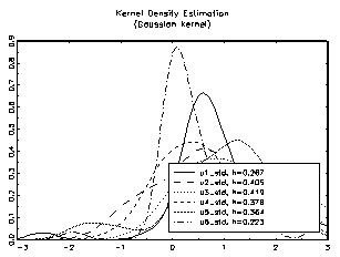
? ? = T -1 ? (? t -? ? )( ? t -? ? ) '(22)and the square matrix ? ? 1/2 is computed. . The standardization of the residuals used here was proposed by Doornik & Hansen (1994) and Lutkepohl (1991). An alternative way of standardization is based on a Choleski decomposition of the residual covariance matrix.
Refer to the appendix (
7. a) Forecasting VECM Processes
Once an adequate model for the data gathering process of a system of variables has been constructed, it may be used for forecasting as well as economic analysis. The concept of Granger-causality, which is based on forecast performance, has received considerable attention in the theoretical and empirical literature. Granger (1969) introduced a causality concept whereby he defines a variable y 2t to be casual for a time series variable y1t if the former helps to improve the forecasts of the latter.
In Table 5 the test for Granger-Causality reveals none of the p-values are smaller than 0.05. Therefore, using a 5% significance level, the null hypothesis of noncausality cannot be rejected. However, in the test for instantaneous causality there is weak evidence of a Granger-causality relation from US productivity differentials ? dollar/euro exchange rate because the p-value of the related test is at least less than 10%.
Table 5 This procedure can be used if the cointegration properties of the system are unknown. If it is known that all variables are at most I(1) , an extra lag may simply be added and the test may be performed on the lagaugmented model. Park & Phillips (1989) and Sims et al (1990) argue that the procedure remains valid if an intercept or other deterministic terms are included in the VAR model. Forecasting vector processes is completely analogous to forecasting univariate processes. It is assumed the parameters are known.
The identification of shocks using restrictions on their long-run effects are popular. In many cases, economic theory suggests that the effects of some shocks are zero in the long-run. Therefore, the shocks have transitory effects with respect to some variables. Such assumptions give rise to nonlinear restrictions on the parameters which may in turn be used to identify the structure of the system.
The impulse responses obtained from a structured VECM usually are highly nonlinear functions of the model parameters. This should be considered when drawing inferences related to the impulse responses.
8. b) Estimation of Structural Parameters
Following the procedure recommended by Lutkepohl (2004), the estimation of the SVAR model is equivalent to the problem of estimating a simultaneous equation model with covariance restrictions. First, consider a model without restrictions on the long-run effects of the shocks. It is assumed that ? t is white noise with ? t ~ N(0, l k ) and the basic model is a VAR; thus the structural form is
A y t = A[A 1 ?..,A p ] Y t-1 + B ? t (23)The concentrated log-likelihood is as follows:
l c (a,B) = constant + T/2 log[A) 2 -T/2 log {B} T/2 m (A'B' -1 A? ?) (24)where
? ? = T -1(Y -A ~Z)(Y -AZY is just the estimated covariance matrix of the VAR residuals as argued by Breitung (2001). Lutkepohl (2004) recommends that continuation of the algorithm stops when some prespecified criterion are met. An example would be a relative change in the log-likelihood and the relative change of the parameters.. The resulting ML estimator is asymptotically efficient and normally distributed, where the asymptotic covariance matrix is estimated by the inverse of the information matrix. Moreover, the ML estimator for ? ?? is
? ? = A ~-1 B ~B~A~-1 (25)Where A ~and B ~ are estimators of A and B, respectively. Note that ? ? ~only corresponds to the In the presence of over-identifying restrictions, an LR test statistic for these restrictions can be constructed in the usual way as LR = T(log l? ? l -log l? ? l) (26)
For VECM'S the concentrated likelihood function
l c (A,B) = constant + T/2 log[A) 2 -T/2 log {B} -T/2 m (A'B' -1 A? ?)(27)* can be used for estimating the structural parameters A and B. If no restrictions are imposed on the short-run parameters, the ?? matrix represents the residual covariance matrix obtained from a reduced rank regression. If the short-run parameters are restricted or restrictions are placed on the cointegration vectors, some other estimator may be used instead of the ML estimator, and ?? may be estimated from the corresponding residuals.
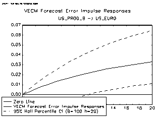
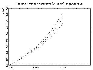
Generally, if long-run identifying restrictions have to be considered, maximization of the above formula is a numerically difficult task because these restrictions are typically highly nonlinear for A, B, or both. In some cases, however, it is possible to express these long-run restrictions as linear restrictions, and maximization can be done using the scoring algorithm defined above. When considering a cointegrated VECM where A = l k, it follows that the restrictions on the system variables can then be written in implicit form as Replacing ? by an estimator obtained from the reduced form we obtain R B,l = R? (l k ? ?, which is a stochastic restriction matrix. These implicit restrictions can be derived. Here t y/2 and t 1-y/2 are the y/2 and (ly/2) equations, respectively, of the empirical distribution of (? -? ) c) Impulse Responses The responses are significant at the 95% level. Table 8 ( in the appendix) displays the point estimates of the impulse responses of the real exchange rate to the one-standard deviation US productivity shocks. Also note that the results are relatively robust with the individual impulse responses falling within the 5% significant tests. Figure 13 shows that for the exchange rate these shocks have a highly significant impact over the 10-year time period and the correlation between these impulse responses is high. They show that productivity shocks have a very significant long-run impact on the dollar/euro exchange rate. The results follow those of Clarida and Galf (1992). The point estimates in table 8 show that for each percentage point in the US-Euro area productivity differential there is a three percentage point real change in the dollar/euro valuation. This suggests that fundamental real factors are significant in the long-run fluctuations in real exchange rates.
Refer to the appendix (figures 31-44) for the US and Euro productivity differentials. Figure 31 shows the long-run impact of productivity shocks on the dollar/euro real exchange rate. Figure 35
9. d) Forecast error variance decomposition
Forecast error variance decomposition is a way of summarizing impulse responses. Following Lutkepohl (2004) the forecast error variance decomposition is based on the orthogonalized impulse responses for which the order of the variables matters. Although the instantaneous residual correlation is small in our subset VECM, it will have some impact on the outcome of a forecast error variance decomposition. Lutkepohl (2004) suggests the forecast error variance as
? 2 k (h) = ?(? 2 kl,n + ?+ ? 2 k,n ) = ? 2 kjo + ?? 2 kh-1 )(30)The term ( 2 kl,n + ?+ ? 2 k,n) is interpreted as the contribution of variable j to the h-step forecast error variance of variables k. This interpretation makes sense if the ? ? s can be viewed as shocks in variable i. Dividing the preceding by ? 2 k (h) gives the percentage contribution of variable j to the h-step forecast error of variable h.
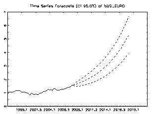
(t) (h) = ? 2 kjo + ?? 2 kh-1/ ? 2 k (h)(31)Chart 1 shows the proportion of forecast error in the dollar/euro accounted for by US productivity, government spending, M2, oil prices and US GDP. The US productivity accounts for 28% over the 20 year time interval with a sharp rise of 21% during the first 5 years. This shows that productivity shocks have a very significant short-run impact on the dollar/euro exchange rate while the long-run impact is more transitory in nature.
10. Discussion of The Results
This paper provides evidence on the long-run relationship between the real dollar/euro exchange rate and productivity measures, controlling for the real price of oil, relative government spending and M2. However, the results imply that the productivity measure can explain only about 27% of the actual amount of depreciation of the euro against the US dollar for the period 1995-2001. This outcome is confirmed by a specification in this study. Figure 18 shows that the productivity can explain only about 28% of the appreciation of the euro during the period 1995-2007 (appendix table 6 for point estimate).
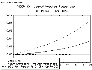
Evidently, productivity is not the only variable affecting the real exchange rate in the model specified. The other variables identified also affected the dollar/euro exchange rate. In particular, the surge in oil prices since early 1999 seems to have contributed to the weakening of the euro. The magnitude of the long-run impact of changes in the real price of oil on the dollar/euro exchange rate is certainly significant. Between 1997 and 2001, the model indicates on the average that the equilibrium euro depreciation related to oil prices developments could have been around 20% (refer to table 8 for point estimate and figure 21). These results are based on long-term relationships.
Overall, the model is surrounded by significant uncertainty, reflecting the inherent difficulty of modeling exchange rate behavior. While we find that in 1995-2001 the euro traded well below the central estimates derived from these specifications, this uncertainty precludes any quantification of the precise amount of over or under valuation at any point in time. This point is also made clear by Detken and Dieppo (2002), who employed a wide range of modeling strategies to show that the deviation from the estimated equilibrium differs widely across models and is surrounded by some uncertainty. Moreover, the results provided by Maeso-Fernandez and Osbat (2001) find various reasonable but nonencompassing specifications leading to different exchange rate equilibria. Again, this suggests a very cautious interpretation of the magnitude of over/under valuation.
11. Year
12. Cusum Tests
The standardization of the residuals used in this model was proposed by Doornik & Hansen (1994) and Lutkepohl (1991). An alternative way of standardization is based on a Choleski decomposition of the residual covariance matrix. Lutkepohl (2004) recommends checking the time invariance of a model by considering recursively estimated quantities. Plotting the recursive estimates together with their standard or confidence intervals can give useful information on possible structural breaks. The recursive estimates of the model are shown in Figures 27-30. They appear to be somewhat erratic at the sample beginning which would reflect greater uncertainty. However, even when taking this into account one finds that the recursive estimates do not indicate parameter uncertainty. The erratic behavior of the recursive estimates at the beginning could be attributed to the change over to the euro in 2001.
The results of the CUSUM tests of the system with 99% level critical bounds (for sample periods 1985-2007) also indicate that government spending, GDP, US productivity, oil prices and M2 recursive estimates are all outside the critical bounds for the CUSUM statistics. This would suggest some stability problems even though they are only outside the critical bounds for the years of 2005-2008. They are all well within the uncritical region for the years up to 2005. For VECMs with cointegrating variables, Hansen & Johansen (1999) have recommended recursive statistics for stability analysis. Figure 35
the tau statistic T( ? r ) is plotted in Figure 36 and the results indicate that the eigenvalue is stable. Therefore, there is no indication of instability of the system appears to be within the 95% confidence intervals. Also,


| Cointegration | Period | Specification | LR Ratios | Critical Ratios |
| Without Oil | & Test Results | |||
| US Prod | 1985-2008 | 2 lags | 3.72 | 16.22*** |
| Euro Prod | 1985-2008 | 2 lags | 2.7 | 12.45** |
| US GDP | 1985-2008 | 2 lags | 2.23 | 12.53** |
| Euro GDP | 1985-2008 | 2 lags | 3.32 | 9.14** |
| US CPI | 1985-2008 | 2 lags | 10.59 | 12.45** |
| Euro CPI | 1985-2008 | 2 lags | 2.48 | 12.45** |
| Table 3 ________________________________________________________________ | ||||
| Cointegration | Period | Specification | LR Ratios | Critical Ratios |
| With Oil | & Test Results | |||
| US Prod | 1985-2008 | 2 lags | 15.34 | 25.73** |
| Euro Prod | 1985-2008 | 2 lags | 31.68 | 42.77** |
| US GDP | 1985-2008 | 2 lags | 13.61 | 16.22*** |
| ) for tests for |
| 8 point estimate | 0.0290 | ||||
| ** Sun, 2 Aug 2009 06:51:29 *** | CI a) | [ 0.0263, 0.0608] | |||
| VAR Orthogonal Impulse Responses | 9 point estimate | 0.0344 | |||
| Selected Confidence Interval (CI): | CI a) | [ 0.0456, 0.0733] | |||
| a) 95% Hall Percentile CI (B=100 h=20) | 10 point estimate | 0.0483 | |||
| Selected Impulse | CI a) | [ 0.0652, 0.0991] | |||
| Responses: "impulse variable -> response | 11 point estimate | 0.0729 | |||
| variable" | CI a) | [ 0.1027, 0.1433] | |||
| time | Oil_prices | 12 point estimate | 0.0895 | ||
| ->US_EURO | CI a) | [ 0.1267, 0.1738] | |||
| point estimate | 0.0000 | 13 point estimate | 0.1251 | ||
| CI a) | [ 0.0000, 0.0000] | CI a) | [ 0.1767, 0.2385] | ||
| 1 point estimate | -0.0354 | 14 point estimate | 0.1593 | ||
| CI a) | [ -0.0653, -0.0469] | CI a) | [ 0.2316, 0.3070] | ||
| 2 point estimate | -0.0174 | 15 point estimate | 0.1827 | ||
| CI a) | [ -0.0401, -0.0183] | CI a) | [ 0.2614, 0.3526] | ||
| 3 point estimate | -0.0111 | 16 point estimate | 0.2337 | ||
| CI a) | [ -0.0322, -0.0085] | CI a) | [ 0.3360, 0.4495] | ||
| 4 point estimate | -0.0027 | 17 point estimate | 0.2849 | ||
| CI a) | [ -0.0187, 0.0035] | CI a) | [ 0.4044, 0.5560] | ||
| 5 point estimate | 0.0017 | 18 point estimate | 0.3500 | ||
| CI a) | [ -0.0113, 0.0109] | CI a) | [ 0.4926, 0.6721] | ||
| 6 point estimate | 0.0086 | 19 point estimate | 0.4260 | ||
| CI a) | [ 0.0030, 0.0251] | CI a) | [ 0.5973, 0.8246] | ||
| 7 point estimate | 0.0054 | 20 point estimate | 0.5119 | ||
| CI a) | [ -0.0036, 0.0243] | CI a) | [ 0.7118, 0.9910] | ||
| Candelon and Lutkepoh (2001) recommended | variables (oil prices and government spending (u4 and | ||||
| using bootstrap versions for the Chow tests to improve | u6). | ||||
| sample properties. The bootstrap is set up with | Lutkepohl (2004) states that if nonnormal | ||||
| modifications to allow for residual vectors rather than | residuals are found, this is often interpreted as a model | ||||
| univariate residual series. Table 9 shows the results of a | defect. However, much of the asymptotic theory on | ||||
| possible break date for 2001 in which the government | which inference in dynamic models is based works also | ||||
| changed to the euro. | for certain nonnormal residual distributions. | Still | |||
| On the basis of the appropriate p-values, the | nonnormal residuals can be a consequence of | ||||
| bootstrap findings of the sample-split. Chow tests do | neglected nonlinearities. Modeling such features as well | ||||
| not reject stability in the model even with the structural | may result in a more satisfactory model with normal | ||||
| break in 2001. | residuals. Sometimes, taking into account ARCH effects | ||||
| Test for Nonnormality The following test for residual autocorrelation is known as the Portmanteau test statistic. The null | may help to resolve the problem. With this in mind a multivariate ARCH-LM test was performed. The results shown in Table 10 indicate the p-value is relatively large: consequently, the diagnostic tests indicate no problem | ||||
| hypothesis of no residual autocorrelation is rejected for large values of Q h (test statistic). The p-value is relatively | with the model. | ||||
| large: consequently, the diagnostic tests indicate no | |||||
| problem with the model. | |||||
| Lomnicki (1961) and Jarque & Bera (1987) | |||||
| propose a test for nonnormality based on the skewness | |||||
| and kurtosis for a distribution. The Jarque & Bera tests | |||||
| in table 9 show some nonnormal residuals for two | |||||