1. Introduction
© 2019 Global Journals purchase a higher fraction of investment products that their advisors were incentivized to sell (promoted products)-see Hackethal et al. 2012. Gennaioli, Shleifer and Vishny focus on the incentives of the money management organization itself when its clients' choices are mediated by trust (see Gennaioli et al., 2015).
These researches rely on Expected utility theory (EUT)(see Neummann and Morgenstern, 1944). However, substantial experimental and empirical evidence reveals that EUT is incompatible with human observed behavior in reality. Demonstrated violations of EUT are as follows.
1) EUT makes the underlying assumption that decision-makers are rational and uniformly risk averse. But, empirical evidence shows that investors' risk attitude often changes.
Specially, Kahneman and Tversky did a experiment to observe changes of personal risk attitude. The first choice is between a sure gain of $240 and a 25% chance to gain $1, 000. The second choice is between a sure loss of $750 and a 75% chance to lose $1,000. For the first choice, 84% of respondents chose a sure gain of $240, which is consistent with risk aversion. For second choice, 87% of respondents chose a 75% chance to lose $1,000, which is consistent with risk seeking. This experiment indicates that people exhibit risk aversion in gains and exhibit risk seeking in losses.
2) EUT generally uses the level of wealth, not changes in wealth. However, in the previous experiment, we find that personal risk attitude changes in the domains of gains and losses. So, we can show that gains and losses seems to be what people care about, rather than the level wealth.
To prove our point of view, we consider the following problem. Decision 1: Assume yourself richer by $300 than you are today. Then, choose between a sure gain of $100 and a 50% chance to gain 200; Decision 2: Assume yourself richer by $500 than you are today. Then choose between a sure loss of $100 and a 50% chance to lose $200. In both cases, the decision is between $400 with certainty and a prospect with a 50% chance of $500 and a %50 chance of $300. Yet, 72% of respondents chose a sure gain of $100 in Decision 1 and 64% chose a 50% chance to lose $200 Decision 2. The choice of many indicates risk aversion for Decision 1, but risk seeking for Decision 2. This problem shows that risk attitude is not same across gains and losses, implying that it is the change in wealth, rather than the level, that matters to people. People evaluate an outcome based on the gain and loss from a reference point, usually taken to be current wealth. Notice that in this problem the two decisions assume different starting wealth positions.EUT cannot incorporate the reference point.
3) Researcher also notice that persons seemed to feel a loss more strongly than gain of equivalent absolute value. But, EUT doesn't involve it.
To more clearly explain our point of view, we consider the following problem. What value of x would make you indifferent between a sure gain of 0 and the prospect which is a 50% chance to gain x and a 50% chance to lose $25? The average of response in this experiment was $61. That is, for a fair gamble, when the loss is $25, the typical person requires a gain of $61 to be indifferent between accepting or rejective the gamble. It is quite clear that people are quite averse to a loss. Loss aversion is the term that describes the observation that, for most people, losses loom larger than gain. 4)EUT cannot explain why a person might buy a lottery ticket and insurance. In fact, overweighting of small probability and subjective probability lead to this behavior.
For example, choose between a 0.1% chance to gain $5,000 and a sure gain of $5. Even though the expected value of the two case are equal ($5) as we almost certainly have observe, many people prefer the former to the latter, consistent with risk seeking, Such a choice is indicative of risk seeking in the domain of gains. Earlier we observed another instance of risk seeking, but this is was in domain of losses. It seems that risk seeking can also occur in the domain of gains as well. Now, we consider another choice. Choose between a 0.1% chance to lose $5,000 and a sure loss of $5. In this case many people choose the latter, consisent with risk aversion. But this implies risk aversion in the negative domain. In sum, while we normally have risk aversion in the positive domain, when there is a quite low probability of a payoff this generally shifts to risk seeking. On the other hand, while we normally have risk seeking in the negative domain, when there is a quite low probability of a loss this generally shifts to risk aversion. This is what Kahneman and Tversky characterized as the fourfold pattern of risk attitudes. This pattern suggests risk aversion for gains and risk seeking for losses when the outcome probability is high, and risk seeking for gains and risk aversion for losses when the outcome probability is low. In onw study, they found that 92%(22 out of 25) of subjects displayed the full patters.
To explain the above violations of EUT and more accurately characterize personal behaviors, Kahneman and Tverskyb propose prospect theory(PT) and cumulative prospect theory (CPT)-see Kahneman and Tversky, 1992a and1992b.
When we research the interaction between investors and managers, we find investors' behavior also deviates from the predictions of EUT. So, in this article, we apply CPTinvestors rather than risk averse investors in the traditional sense. That is, we adopt a cumulative prospect theory (CPT) approach to the investor's preferences. In a original way, we model the investor's trust in the manager and associated anxiety from investing in a risky asset to determine a CPT investor's optimal portfolio and a manager's optimal fees.
The novelty of our contribution relative to Gennaioli et al.( 2015) and other works using classical preferences is that we rely on cumulative prospect theory rather than the classical mean-variance framework. Gennaioli, Shleifer and Vishny (2015) assume that all investors are rational. Hence, they develop a model relying on the mean-variance framework, which is certainly the most well-known investment decision rule. However, all of our investors are CPT investors, namely, these investors' behavior coincides with cumulative prospect theory. Specifically, we employ a value function for CPT investors, while Gennaioli, Shleifer and Vishny (2015)use a classical utility function. In the value function of our CPT investors, we consider the gain relative to a reference wealth level, i.e., the benchmark wealth. However, Gennaioli et al. (2015)use absolute wealth in the investors' utility function. Moreover, to accurately characterize a CPT investor's psychology, we combine probability distortions with the value functions to measure the CPT investors' satisfaction, while Gennaioli, Shleifer and Vishny (2015)use only a simple probability and the investors' utility functions to measure investor satisfaction. In other words, Gennaioli et al.(2015) only employ the expected utility functions to measure investor satisfaction. The value function and probability distortions are the key contributions of cumulative prospect theory and allow our CPT model to outperform traditional theory in real financial markets.
Another innovation is that we focus on the dynamic portfolio selection but not the static portfolio choices. Gennaioli et al. only discuss the managers' optimal fees when the investors invest in the risky asset in a single period. However, we explore the managers' optimal fees and the investor's portfolio selection under multi-period setting. Moreover, based on the subgame perfect investment strategies, we obtain the CPT investor's optimal portfolio in multi-period.
In their analysis of multiple financial products, Gennaioli et al. (2015)only consider two risky assets, while we study two or more such assets. Moreover, their research relies on the assumption that the two risky assets are uncorrelated, an assumption that we need not make.
There are two main differences between our results and those based on classical preferences. First, in our results, the optimal fees are not symmetric. In particular, the dominant managers obtain a higher fee than do subordinate managers regardless of the changes in risk of risky assets (a risky asset) and the changes in the dispersion of trust in the population. Another difference is that, in our work, these fees are not proportional to expected returns. Moreover, the optimal fees decline nonlinearly as risk of risky assets (a risky asset) decreases and the dispersion of trust in the population decreases.
Except for our application of CPT in money doctor, CPT is applied extensively in the contexts of optimal investment strategy and optimal insurance contracts.
Regarding optimal investment strategy, in a continuous-time setting, Jin and Zhou (2008) formulate a general behavioral portfolio selection model using Kahneman and Tversky's CPT. In a discrete-time setting, Bernard and Ghossoub (2009) consider how a CPT investor chooses his/her optimal portfolio in a single-period model with one risky and one riskless asset. In the same vein, He and Zhou (2011a,b) address and formulate the general well-posedness issue and investigate the case in which the reference point is not the risk-free return. Pirvu and Schulze (2012) extend this work to a multi-asset context. To the best of our knowledge, Shi et al. (2014) are the first to consider the CPT allocation problem in a multi-period framework. Deng and Pirvu investigate optimal portfolio selection with one risk-free asset and one risky asset in a multi-period setting under CPT (see Deng and Pirvu, 2015). Compared with Shi et al's study, their novelty is that the optimal strategies are time inconsistent due to the time-changing benchmark.
Regarding optimal insurance contracts, there are fewer results (and those that exist are less sophisticated) than in the context of optimal portfolio choice. From the insured's perspective, Dhiab investigates the demand for insurance under CPT (see Dhiab, 2015). From the insurer's perspective, Bernard et al. explore the optimal insurance policy for an insurer with a linear cost function (see Bernard et al., 2015). Based on Bernard et al.'s work, Deng identifies the optimal insurance policy for the more general insurer cost functions, addressing both linear and nonlinear cost functions (see .
Although CPT is more practical than traditional models, it is not more widely used than traditional theory. As noted above, CPT is applied primarily to address problems related to optimal investment strategy and optimal insurance contracts. To the best of our knowledge, for many other other problems related to CPT, in particular the optimal fees that managers charge under CPT, there are no existing studies. This lack of research is certainly not because this problem is unimportant or uninteresting; rather, we believe, this lack of research is because addressing such problems using CPT is considerably more complicated than doing so using the traditional decision optimization.
In extant CPT research, researchers only consider the value function of a CPT investor who invests in a risky asset without assistance. Moreover, they focus solely on the optimal portfolio for the investor. However, we are interested in investors' interaction with portfolio managers and thus develop a value function for a CPT investor investing in risky assets with the assistance of a portfolio manager, not on his own. Our models accurately characterize and reflect the reduced anxiety experienced by CPT investors when bearing risk with the assistance of a trusted portfolio manager. Moreover, we determine not only the investor's optimal portfolio but also the money managers' optimal fees. However, our original models pose an enormous computational challenge, as the traditional method is not suitable for our new problem. To overcome these computational difficulties, we use rigorous derivation to obtain the implicit solutions. Then, we employ an effective software tool and obtain approximately explicit solutions. The remainder of this paper is organized as follows. In Section 2, we discuss a basic setting. In section 3, we attain the CPT investor's optimal portfolio in multi-period under CPT. In section 4, we investigate managers' total profits. In section 5, we determine the optimal fees charged by money managers. Section 6 contains the numerical analysis. In Section 7, we compare our results with those of Gennaioli et al. and explain our results from an economic perspective. The paper concludes with an Appendix containing the proofs.
2. II.
3. The Basic Setup
In this paper, we analyze the dynamic optimal strategies. We consider a financial market in which the CPT-investor can invest in one risk-free asset and one risky asset. The investing horizon is [0, T ], where T is a finite deterministic constant. The time of investment t takes on discrete values (t = 0, 1, ..., T ? 1). Moreover r t denotes the return of the risk-free asset from the time t to the time t + 1, and x t denotes the return of the risky asset from the time t to the time t + 1. We assume that a CPT-investor i has wealth W i,t at the time t and invest the amount v i,t in the risky asset and all of remaining wealth W i,t ? v i,t in the risk-free asset. The investor's wealth W i,t+1 at time t + 1 is given by the equation
W i,t+1 = (1 + r t )(W i,t ? v i,t ) + (1 + x t )v i,t = (1 + r t )W i,t + y t v i,t .(2.1)
Here y t = x t ?r t is a random variable and represents the excess return on the risky asset over the risk-free asset from the time t to the time t + 1. The excess return {y t } {t=0,1,...,T ?1} is an adapted stochastic process defined over the probability space (?, F t , F, P ). The information set at the beginning of period t is denoted as F t = ?(y 0 , y 1 , ..., y t?1 ). Besides, assume the variance of the excess return is ? 2 and the expected value of the excess return is µ.
A CPT-invest doesn't feel anxious when he invests in the risk-free asset. However, the CPT-investor feels anxious and nervous when he invests in the risky asset. The reason is that the CPT-invest should not only have professional knowledge and relevant information but also spend much time and energy on the analysis of portfolio in order to attain a satisfied return of the risky asset. But it is very difficult for an average CPT-investor to do these. Thus, the CPT-investor is willing to invest in the risky asset on a trusted and experienced wealth manager rather than on his own. In a pure mathematical sense, this assumption is not very strict, but it clearly presents the foundation and background of our research and makes the practical meanings of our result more explicit. As the viewpoint of Gennaioli, Shieifer and Vishny, a money manager plays a similar role in the financial market to a doctor. In particular, almost of investors do not know how to invest expect for the investment in a risk-free asset, so they want to seek some financial advice from a trusted and experienced manager. It is like that almost of patients have little idea of how to be treated but some simple and safe treatments, thus they prefer to seek some medical advice from an expert and trusted doctor. The present article discusses the similar problem that CPT-investors invest in a risk asset on a trusted money manager but not on their own. Actually, the relationship between the CPT-investors and the money managers in our research is also like the relationship between the patients and the doctors.
Each of the manager who the CPT-investor i can choose is denoted by j. In general, j = 1, 2, 3, .... The CPT-investor delegates his wealth management to the portfolio manager who this investor most trusts. We add the element of trust to the traditional value function of a CPT-investor. Denoted by ? i,j ? [0, 1] the investor i's level of trust on the money manager j. The higher ? i,j represents that the investor puts more trust in the manager j and the investor i suffers less anxiety when he invests his wealth in a risky asset with the manager j. The fee rate charged by money manager j is denoted by f j . Let a i,j = a? i,j , where a is a nonnegative constant. Indeed, a i,j is the measure of the CPT-investor i's anxiety when he hires the manager j. a represents the measure of the CPT-investor i's anxiety when he hires the most trusted manager. The idea will be specially formalize in the next section.
In this paper, we only consider a simple case in which the CPT-investor hires one of two managers, A or B. So, in the section 2.3, we directly set j = A and j = B. We suppose that half of the CPT-investors trust the manager A more than the manager B. These investors are denoted by A-trusting investors. Similarly, there are half of the CPT-investors trusting the manager B more than the manager A, who are called B-trusting investors. The anxiety which an A-investor suffers when he invests in the risky asset on the manager A equals a. To similar, the anxiety suffered by a B-investor for bearing risky with the manager B's financial advice is also a. It can differ from different CPT-investors how much they trust one manager over the other. Particularly, in the population of CPT-investors ? i satisfies uniformly distributed on [1 ? ?, 1] for both A-trusting investors and B-trusting investors, where parameter ? ? [0, 1] captures the dispersion of trust in the population. The lower is ?, the less investors trust one manager more than the other. When ? = 0, the investor trusts one manager as much as the other. This dispersion in trust level makes the money managers gain respect of the CPT-investors who trust these managers more. And, these managers can charge the optimal and positive fees even in a competitive financial market. The trust is permanent and does not depend on the change of returns.
Simply speaking, we consider the following the optimal problems. Two managers A and B decide the optimal fees at the time t (t = 0, 1, ..., T ? 1) in order to attract the CPTinvestors and gain most total profits in competition at the time T . From the CPT-investors' standpoint, at the time t, the investors choose the optimal portfolio in order to maximize their own objective function at the time T .
4. III.
The Model
a) The Benchmarked Wealth Let R k t = ? k?1 j=t (1 + r j )(0 ? t ? T ? 1, 1 ? k ? T ), with k ? t be the value of 1 dollar (in the portfolio at time t) at time k. If the initial time is t, we let the benchmark be R k t W i,t at the time k (this is the amount at time k of W t invested in the risk free asset at time t). The benchmarked wealth at time t + 1, given initial time t is
W t+1 i,t = R t+1 t W i,t + y t v i,t ? R t+1 t W i,t = y t v i,t . (3.1)Given the initial time t the benchmarked wealth at time t + 2 is
W t+2 i,t = R t+2 t+1 W i,t+1 + y t+1 v i,t+1 ? R t+2 t W i,t = R t+2 t+1 y t v i,t + y t+1 v i,t+1 . (3.2)Generally, we let the initial time be t (t=0,1,2,...,T-1). We can characterize the benchmarked wealth at the end of the investment horizon by the following Proposition.
W T i,t = R T t+1 v i,t y t + R T t+2 v i,t+1 y t+1 + ... + R T T ?1 v i,T ?2 y T ?2 + v i,T ?1 y T ?1 . (3.u i,j (W T i,t , a i,j ) (3.4) = { u + i,j (W T i,t ) = u + (W T i,t ? f j + a? i,j ? 2 ) = (W T i,t ? f j + a? i,j ? 2 ) ? W T i,t ? 0, u ? i,j (?W T i,t ) = ?u ? (?(W T i,t ? f j + a? i,j ? 2 )) = ??(?W T i,t + f j ? a? i,j ? 2 ) ? W T i,t < 0.It is worth stressing that a i,j has a different meaning from that used by Gennaioli et al. In our model, a i,j is the measure of CPT investor i's trust when he hires manager j. In particular, a represents a measure of CPT investor i's anxiety when he hires his most trusted manager. However, in Gennaioli et al.'s model, a i,j is the measure of CPT investor i's anxiety when he hires manager j:
u i,j (c) = E(c) ? a i,j 2 V ar(c)This different meaning is attributable to different reference levels. In our model, a i,j , as a measure of trust, makes the value function of a risk-averse investor without a manager's help, W ? i , increase to that of a risk-averse investor with a manager's help, (W i ? f j + a? i,j ? 2 ) ? . In other words, we take the value function of a risk-averse investor without a manager's help, W ? i , as a reference level. In Gennaioli et al.'s model, a i,j , as a measure of anxiety, makes the value function of a risk-neutral investor E(c) decrease to that of a risk-averse investor, E(c) ? a i,j 2 V ar(c). In other words, they take the value function of a risk-neutral Definition 3.1. (see Tversky and Kahneman (1992a) and Tversky and Kahneman (1992b))The value function u is defined as follows:
u(x) = { u + (x) if x ? 0 , ?u ? (?x) if x < 0,where u + : R + ? R + and u ? : R + ? R + satisfy:
(i) u(0) = u + (0) = u ? (0) = 0; (ii)u + (+?) = u ? (+?) = +?; (iii)u + (x) = x ? , with 0 < ? < 1 and x ? 0; (iv)u ? (x) = ?x ? , with ? > 1 and x ? 0.Definition 3.2. Let F W (?) be the cumulative distribution function (CDF) of a random variable W . We define the two probability weight functions (distortions)
T + : [0, 1] ? [0, 1] and T ? : [0, 1] ? [0, 1]as follows:
T + (F W (x)) = F ? W (x) (F ? W (x) + (1 ? F ? W (x)) ? ) 1/? , with 0.28 < ? < 1 T ? (F W (x)) = F ? W (x) (F ? W (x) + (1 ? F ? W (x)) ? ) 1/? , with 0.28 < ? < 1.When the CPT investor is risk averse, he feels less anxious and nervous about bearing the risk when he has the assistance of a trusted and experienced money manager. The CPT investor is only risk averse when the benchmark wealth is nonnegative, i.e., x ? 0. When x < 0, the CPT investor is risk seeking. Thus, we only need to modify value function u + and can leave value function u ? unchanged.
investor, E(c), as a reference level. If we examine the value function of a risk-averse investor
a i,j 2 .Here, trust (? i,j /a i,j ) relates to the advertisements for money manager j, money manager j's services for investor i, investor i's investment experience, and investor i's educational background, among others. However, trust does not depend on the riskiness of risky assets. Therefore, when manager j invests in riskier projects, investor i's level of trust in manager j remains the same. This assumption is consistent with that of Gennaioli et al.
We assume that the anxiety suffered by CPT investor i for bearing the risk with the assistance of any manager j is less than it would be if he were to invest on his own, even if manager j is not CPT investor i's most trusted manager. That is, we suppose that
a? i,j ? 2 ? f j ? 0. (3.5)To clearly explain our model, we introduce the subjective risk premium as Davies and Satchell involved (see Davies and Satchell , 2004). Denote the probability of a gain by p.
The subjective premium, ?, is defined as
u i,j (E s (W T i,t ) ? ?) = (1 ? p)E[u ? i,j (W T i,t )m ? (W T i,t )|W T i,t < 0] + pE[u + i,j (W T i,t )m ? (W T i,t )|W T i,t > 0],(3.6)where
m + (W T i,t ) = (T + ) ? (F W T i,t (x)), m ? (W T i,t ) = (T ? ) ? (F W T i,t (x)), E s (W T i,t ) = ? +? 0 x(T + ) ? (F W T i,t (x))dx + ? 0 ?? x(T ? ) ? (F W T i,t (x))dxand E[?] is a expected value in a traditional sense. We compare a subjective risk premium for no manager's help with that for a manager's help. Denote the former by ? 0 and latter by ?. Proposition 3.2. When CPT investor i is risk averse, that is, ? > 0. CPT investor i face a gamble with outcomes distributed according a random benchmarked wealth. Then, the manager's help can reduce his anxiety, that is, ? < ? 0 .
We prove this in Appendix A. Let
G1 = (u ? i,j ) ? (0)m ? (??), H1 = 1 2 ( (u ? i,j ) ?? (0)m ? (??) + (u ? i,j ) ? (0)(m ? ) ? (??) ) , G2 = (u + i,j ) ? (0)m ? (??), H2 = 12( (u + i,j ) ?? (0)m ? (??) + (u + i,j ) ? (0)(m ? ) ? (??) ) , G3 = (u + i,j ) ? (?)m + (0) + u + i,j (?)(m + 0) ? (0),Global( (u + i,j ) ?? (?)m + (0) + 2(u + i,j ) ? (?)(m + ) ? (0) + u + i,j (?)(m + ) ?? (0)) ,
I = u + i,j (?)m + (0). (3.7)We can obtain the following proposition about risk premiums.
Proposition 3.3. If E s (W T i,t ) ? 0, E(W T i,t ) ? 0 and G1 u ? i,j (0) > 0, H1 u ? i,j (0) < 0, G2 u ? i,j (0) < 0, H2 u ? i,j (0) < 0, I u ? i,j (0) < 0, G3 u ? i,j (0) < 0, H3 u ? i,j (0) < 0,then the objective risk premium is positive, that is, CPT investor i is locally risk aversion. Moreover, the subjective risk premium is positive, ? > 0, that is, he believes himself to be risk aversion.
We prove this in Appendix B.
Definition 3.4. Define the objective function of the CPT-investor at the time t, denoted by U (W T i,t , f j ), as:
U (W T i,t , f j ) = ? +? 0 T + (1 ? F W T i,t (x))du + i,j (x) + ? 0 ?? T ? (F W T i,t (x))du ? i,j (?x) (3.8)where W T i,t is the benchmark wealth. U (W T i,t , f j ) is a sum of two Choguet integrals (see Choquet (1953) and Chateauneuf et al. (2000)). It is well-defined when ? < 2 min(?, ?).
In this section we formulate the CPT investor objective. Since the benchmark at the end of investment horizon is R T t W i,t , it is changing with respect to t. This makes optimal strategies time inconsistent. Due to this predicament we consider sub game perfect strategies which are formally defined below.
We first consider the optimal problem on the time period [T ? 1, T ]. At the time T ? 1, we discuss the optimal problem (P 1) :
sup v i,T ?1 ?R + U (W T i,T ?1 (v i,T ?1 ), f j ) = sup v i,T ?1 ?R + [ ? +? 0 T (1 ? F W T i,T ?1 (x))du + i,j (x) + ? 0 ?? T ? (F W T i,T ?1 (x))du ? i,j (?x)] .
(3.9)
5. c) Characterization of the Optimal Portfolio Choices
And, we can obtain the optimal solution of (P 1)
v * i,T ?1 = arg max v i,T ?1 ?R + U (W T i,T ?1 (v T ?1 ), f j ) = arg max v i,T ?1 ?R + [ ? +? 0 T (1 ? F W T i,T ?1 (x))du + i,j (x) + ? 0 ?? T ? (F W T i,T ?1 (x))du ? i,j (?x)] .
(3.10) Applying policy iteration to the more general time period [t, T ] (t = 0, 1, ..., T ? 1), we seek the subgame perfect investment strategies
©V i,t = { v * i,k k=t+1,t+2,...,T-1, v i,k 0, k=t,for an arbitrary F t -adapted control v i,t .
At the time t, we consider the optimal problem
(P n) : max V i,t U (W T i,t , f j ) = max V i,t [ ? +? 0 T (1 ? F W T i,t (x))du + i,j (x) + ? 0 ?? T ? (F W T i,t (x))du ? i,j (?x)] .
(3.11) And, we have the optimal solution of (P n)
V * i,t = (v * i,t , v * i,2 , ..., v * i,T ?1 ) = arg max V i,t U (W T i,t , f j ) = arg max V i,t [ ? +? 0 T (1 ? F W T i,t (x))du + i,j (x) + ? 0 ?? T ? (F W T i,t (x))du ? i,j (?x)] .
(3.12)
The optimal time consistent strategy is
V * i,0 = (v * i,0 , v * i,1 , ..., v * i,T ).6. d) The Portfolio Optimization
We get a important result for the optimal fees of managers.
Theorem 3.4. Given that V i,t > 0 (no short-selling), the subgame perfect CPT-investment strategy is given by
V * i,0 = (v * 0 , v * 1 , ..., v * T ), where v * i,t = { k * i,t ( a? i,j ? 2 ? f j )W i,t W i,t ? 0 k * i,t ( a? i,j ? 2 ? f j )W i,t W i,t < 0 (3.13)where
k * i,t = arg max z?0 G i,t (z), k * i,t = arg max z<0 L i,t (z) G i,t (z) = E[(1 + r t + zy t ) ? A i,t+1 I 1+rt+zyt?0 ? (?1 ? r t ? zy t ) ? B i,t+1 I 1+rt+zyt<0 F T ?2 ] (t = 0, 1, ..., T ? 2), L i,t (z) = E[(?1 ? r t ? zy t ) ? A i,t+1 I 1+rt+zyt?0 ? (1 + r t + zy t ) ? B i,t+1 I 1+rt+zyt>0 F t ] (t = 0, 1, ..., T ? 2), G i,T ?1 (z) = ? +? 0 T + (1 ? F y T ?1 (y))?(zy + 1 W i,T 1 ) ??? ? 0 ?? T ? (F y T ?1 (y))??(?zy) ??1 zdy, L i,T ?1 (z) = ? +? 0 T + (1 ? F y T ?1 (y))?(?zy + 1 W i,T ?1 ) ??1 zdy ? ? 0 ?? T ? (F y T ?1 (y))??(zy) ??1 zdy, A i,t = max z?0 G i,t (z), (t = 0, 1, ...T ? 1) B i,t = ? max z<0 L i,t (z) (t = 0, 1, ...T ? 1).We prove this in Appendix C.
IV.
7. The Objective
Here, we only consider two managers, A and B. If investor i has greater trust in manager A than in manager B, then
? i,A = 1. ? i,B is uniformly distributed on [1 ? ?, 1], where the parameter ? ? [0, 1] captures the dispersion of trust in the population. Here, we call investor i an A-trusting investor. Analogously, there are other investors called B-trusting investors, who trust manager B more than manager A. In the following section, we will discuss the total profit of manager A. We first discuss the total profit of manager A when
f A ? f B . If max v i,t ?R U (W T i,t , f A ) ? max v i,t ?R U (W T i,t , f B ),investor i prefers manager A to manager B. Similar to the results in Deng (2015), we have
( a? i,A ? 2 ? f A ) ? (W ? i,t A i,t I Wt?0 ? ( a? i,j ? 2 ? f j ) ? (?W i,t ) ? B i,t I Wt<0 ) ? ( a? i,B ? 2 ? f B ) ? (W ? i,t A i,t I Wt?0 ? ( a? i,j ? 2 ? f j ) ? (?W i,t ) ? B i,t I Wt<0 ).Thus,
a ? 2 (? i,A ? ? i,B ) ? (f A ? f B ). (4.1)Note that the right-hand side of (4.1) is not less than 0. For B-trusting investors, the left-hand side of (4.1) is less than 0. Thus, (4.1) does not hold. That is, none of the B-trusting investors will choose manager A.
For an A-trusting investor, if
? i,B ? 1 ? ? 2 a (f A ? f B ),the A-trusting investor prefers manager B. Namely, although manager A charges a higher fee than manager B, some A-trusting investors have so little trust in manager B that they prefer manager A, regardless of manager A's higher fee. Hence, when f A ? f B , given Theorem 3.4, we can state that the manager A obtains total profit
8. Global Journal of Management and Business Research
Volume XIX Issue V Version I Year 2019 ( )
C Dynamic Money Doctors under Cumulative Prospect Theory f A ( a ? 2 ? f A )W i,t (k * i,t I W i,t ?0 + k * i,t I W i,t <0 ) ? max[1??, ? 2 a f B ,1? ? 2 a (f A ?f B )] max[1??, ? 2 a f B ] 1 2? d? i,B = f A ( a ? 2 ? f A )W i,t (k * i,t I W i,t ?0 + k * i,t I W i,t <0 ) ? max[1??,1? ? 2 a (f A ?f B )] max[1??, ? 2 a f B ] 1 2? d? i,B .In fact, we can demonstrate that 1 ? ? ? ? 2 a f B . Otherwise, there would be some paradoxical results. Specifically, when 1
? ? < ? 2 a f B , if exits any ? i,B ? [1 ? ?, ? 2 a f B ], then this is inconsistent with equation (3.5). If no ? i,B satisfies ? i,B ? [1 ? ?, ? 2 a f B ], namely, any ? i,B ? [ ? 2 a f B , 1], this contradicts the assumption that ? i,B is uniformly distributed on [1 ? ?, 1]. Thus, 1 ? ? ? ? 2 a f B is reasonable. Moreover, if max v i,t ?R U (W T i,t , f B ) ? max v i,t ?R U (W T i,t , f A ), namely, a ? 2 (? i,B ? ? i,A ) ? (f B ? f A ),(4.2)the investor i prefers manager B to manager A.
Since
? i,A ? ? i,B ? [??, ?], equation (4.2) indicates that ? 2 a (f B ? f A ) ? ??.Otherwise, the equation (4.2) will always hold and the CPT-investor i will always prefer the manager B. Then, manager A earns zero profit. Manager A could reduce his fee and make positive profits.
When
f A ? f B , manager A's total profit U f A (f A , f B ) is rewritten as U A (f A , f B ) = f A ( a ? 2 ? f A )W i,t (k * i,t I W i,t ?0 + k * i,t I W i,t <0 ) ? 1? ? 2 a (f A ?f B ) 1?? 1 2? d? i,B .9. Subsequently, we consider f
investor i prefers manager A to manager B. From
( a? i,A ? 2 ? f A ) ? (W ? i,t A i,t I Wt?0 ? (?W i,t ) ? B i,t I Wt<0 ) ? ( a? i,B ? 2 ? f B ) ? (W ? i,t A i,t I Wt?0 ? (?W i,t ) ? B i,t I Wt<0 ).we can demonstrate that If investor i is an A-trusting investor, as mentioned above, ? i,A = 1. Hence, ? i,A ?? i,B ? 0. Since the right-hand of (4.3) is less than 0, (4.1) always holds. Therefore, all A-trusting investors prefer manager A.
a ? 2 (? i,A ? ? i,B ) ? (f A ? f B ). (4For a B-trusting investor and when ? i,B = 1, if
? i,A ? 1 + ? 2 a (f A ? f B ),a B-trusting investor will choose manager A, as he hopes to pay less in management fees. Therefore, when f B > f A , manager A's total profit is
f A W i,t (k * i,t I W i,t ?0 + k * i,t I W i,t <0 )[ 1 2 ( a ? 2 ? f A ) + ? 1 max[1??,1+ ? 2 a (f A ?f B )] ( a? i,A ? 2 ? f A ) 1 2? d? i,A ].(4.4) From equation (4.3), we have that
? 2 a (f A ? f B ) ? ??. That is, max[1 ? ?, 1 + ? 2 a (f A ? f B )] = 1 + ? 2 a (f A ? f B ). Therefore, when f B > f A , manager A's total profit U f A (f A , f B ) is U A (f A , f B ) = f A W i,t (k * i,t I W i,t ?0 + k * i,t I W i,t <0 )[ 1 2 ( a ? 2 ? f A ) + ? 1 1+ ? 2 a (f A ?f B ) ( a? i,A ? 2 ? f A ) 1 2? d? i,A ]. (4.5)As for the above results, we can obtain the manager A's total profits U A (f A , f B ) by
U A (f A , f B ) (4.6) = ? ? ? ? ? ? ? f A ( a ? 2 ? f A )W i,t (k * i,t I W i,t ?0 + k * i,t I W i,t <0 ) ? 1? ? 2 a (f A ?f B ) 1?? 1 2? d? i,B . if f A ? f B , f A W i,t (k * i,t I W i,t ?0 + k * i,t I W i,t <0 ) ?[ 1 2 ( a ? 2 ? f A ) + ? 1 1+ ? 2 a (f A ?f B ) ( a? i,A ? 2 ? f A ) 1 2? d? i,A ]. if f A < f B .Similarly, the total profit U B (f A , f B ) of manager B is given by
U B (f A , f B ) (4.7) = ? ? ? ? ? ? ? f B ( a ? 2 ? f B )W i,t (k * i,t I W i,t ?0 + k * i,t I W i,t <0 ) ? 1? ? 2 a (f B ?f A ) 1?? 1 2? d? i,A . if f B > f A , f B W i,t (k * i,t I W i,t ?0 + k * i,t I W i,t <0 ) ?[ 1 2 ( a ? 2 ? f B ) + ? 1 1+ ? 2 a (f B ?f A ) ( a? i,B ? 2 ? f B ) 1 2? d? i,B ]. if f B ? f A .The above results lead us directly to the key theorem below.
Theorem 4.1. Suppose that ? i,B is uniformly distributed on [1 ? ?, 1], where the parameter ? ? [0, 1] captures the dispersion of trust in the population. If the managers provide a service for the investors, all of whom behave according to CPT, namely, all are CPT investors, we can characterize manager A's the total profit U A (f A , f B ) by
U A (f A , f B ) (4.8) = ? ? ? ? ? f A ( a ? 2 ? f A )W i,t (k * i,t I W i,t ?0 + k * i,t I W i,t <0 ) 1 2? (? ? ? 2 a (f A ? f B )) if f A ? f B , f A W i,t (k * i,t I W i,t ?0 + k * i,t I W i,t <0 ) ?[ 1 2 ( a ? 2 ? f A ) + 1 4? (2 ? ? 2 a f B ? ? 2 a f A )(f B ? f A )] if f A < f B ,and manager B's total profit U B (f A , f B ) by
U B (f A , f B ) (4.9) = ? ? ? ? ? f B ( a ? 2 ? f B )W i,t (k * i,t I W i,t ?0 + k * i,t I W i,t <0 ) 1 2? (? ? ? 2 a (f B ? f A )) if f B > f A , f B W i,t (k * i,t I W i,t ?0 + k * i,t I W i,t <0 ) ?[ 1 2 ( a ? 2 ? f B ) + 1 4? (2 ? ? 2 a f A ? ? 2 a f B )(f A ? f B )] if f B ? f A ,.(4.10)
V.
10. The Results
This identifies the optimal fees in two different cases, one in which the dominant manager is manager A and the other in which the dominant manager is manager B.
Proposition 5.1. We set
f * A = arg max f A U A (f A , f B )and
f * B = arg max f B U B (f * A , f B ).11. If manager A is in a dominant position and manger B is in a subordinate position in the financial market, then f
and
f * B = 2? + 2 ? x ? ? (2? + 2 ? x) 2 ? 4(? + 1 2 (1 ? x 2 )) 2? 2 /a , (5.2)where
x = 1 ? ? 2 a (f * A ? f * B ).The approximately and explicitly optimal solutions of f * A and f * B are as follows
f * A = C + D a ? 2 (5.3)and
f * B = E + F a ? 2 , (5.4)where
C = 2? + 2(2? + 1) 1/2 ? 1 > 0,(5.5)12. Global Journal of Management and Business Research
Volume XIX Issue V Version I Year 2019 ( )
C Dynamic Money Doctors under Cumulative Prospect Theory D = 1 2 [8(? ? 1)(2? + 1) 1/2 + 4? 2 + 3],(5.6)E = 1 2 (4? ? 2 + 4(2? + 1) 1/2 ) > 0 (5.7)and
F = 1 2 ((8? ? 6)(2? + 1) 1/2 + 4? 2 +). (5.8)If manager B is in a dominant position and manger A is in a subordinate position in the financial market, we obtain the symmetrical results.
The proof of this proposition is seen in Appendix D.
It is valuable to notice that the result coincides with the static result (see ). Here, we must stress that Gennaioli et al.'s f A and f B are the rates of fees while our f A and f B are the amounts of fees. To more clearly compare our results with those of Gennaioli et al., we calculate the rates of fees in our model and attain the following proposition.
13. Proposition 5.2. Let the rates of fees be
(5.9)
In addition, set
F * A = arg max F A U A (F A , F * B )and
F * B = arg max F B U B (F * A , F B ).If manager A is in a dominant position and manager B is in a subordinate position in the financial market, then
F * A = ? 1 k? + 1 k?(1 ? C ? 2 a ) + D (5.10)and
F * B = ? 1 k? + 1 k?(1 ? E ? 2 a ) + F . (5.11)Conversely, if manager B is in a dominant position and manager A is in a subordinate position in the financial market, then
F * B = ? 1 k? + 1 k?(1 ? C ? 2 a ) + D (5.12)and
F * A = ? 1 k? + 1 k?(1 ? E ? 2 a ) + F . (5.13)Moreover, both F * A and F * B are increasing functions of ? 2 . That is, a riskier asset commands higher rates of fees, such that managers are willing to take on market risk.
The proof of this proposition is provided in Appendix E. Although managers serve CPT investors rather than risk-averse investors in the classical theory, they also charge higher rates for riskier assets. This mechanism is consistent with that of Gennaioli et al.
Remark 5.1. Proposition 5.2 indicates that the rates of net fees are higher for riskier assets. We find that the rates of gross fees are also higher for riskier assets. Given that GF j is the amount of the gross fee, we can obtain the rate of the gross fee, GF j , as follows:
GF j = a? i,j ? 2 + f j W i = ? 1 k? + 2 k? 1 1 + D ? C ? 2 a? i,j.
(
Hence,
?GF j ?? 2 = 2 k? C a? i,j (1 + D ? C? 2 a? i,j ) ?2 > 0. (5.15)Therefore, GF j is an increasing function of ? 2 . That is, the rate of the gross fee is also higher for riskier assets.
From above results, we find that the optimal fees obtained for the dominant managers are not very satisfactory because the optimal solutions are implicit, not explicit. This shortcoming is always a major obstacle to the application of CPT. To nullify this disadvantage, we use an effective software program to obtain the above approximately explicit solution. However, the explicit solution is so complicated that we cannot clearly analyze the relationship between the managers' optimal fees and the various parameters. Therefore, we will describe this relationship using numerical analysis.
14. VI.
15. Numerical Analysis
In this section, under the assumption that all of the investors are CPT investors served by either manager A or B, we focus primarily on the optimal problem for multiple stocks. The single-stock problem is similar to the multiple-stock problem, except that ? is replaced with ?. We assume that manager A is in the dominant position in and the manager B is in the subordinate position. We examine how the parameter ?2 a affects the strategies of managers A and B. increases. When a ?2 increases from 0 to 5.0, manager A's fee declines to 5% from 30% while manager B's fee declines to 5% from 25%. When increasing the parameter a ?2 , the decrease in the index ?2 reflects the less risks associated with the portfolio of the risky assets. Hence, from the managers' perspective, manager A (who is in the dominant position) only need lower rates of fees to take risk. Manager B (who is in the subordinate position) has to reduce his fees to compete with manager A and earn a profit. ii) Manager A (who, again, is in a dominant position) charges a higher fee than the subordinate manager B. The highest fee charged by manger A is approximately 30%, while the highest fee charged by manger B is approximately 25%. iii) The parameter ? slightly affects the optimal fees. For fixed a ?2 = 5.0, when ? increases by 1.0 from 0.5, manager A's fee increases from 5.0 to approximately 9.0 whereas manager B's fee increases to 8.0 from 5.0. a increases from 0 to 5.0, manager A's total profit increases to 0.98 from 0 while manager B's total profit increases to 0.34 from 0. Note that when ?2 a = 0, the total profits of manager A and manager B are both 0. This reason is that ?2 a = 0 means the risk associated with the portfolio of risky assets is quite small, and thus, CPT investors prefer to invest on their own instead of with money managers. Note further that when relating the fees to the total profits, total profits increase when the fees decline. This signifies that a strategy of reducing fees would be effective in the financial market. Although the managers charge lower fees when ?2 a increases, the total profits increase because lower fees attract more CPT investors. ii) Manager A (who is in a dominant position) obtains more total profits than the manger in the subordinate position. For fixed ? = 0.5, the largest total profit for manger A is approximately 0.98 while the largest total profit for manger B is approximately 0.34. iii) The parameter ? has a greater influence on manager B's total profit than on manager A's total profit. For fixed ?2 a = 5.0, when ? increases by 1.0 from 0.5, manager B's total profit falls from 0.34 to approximately 0.18 whereas manager A's total profit declines from 0.98 to 0.95.
16. VII.
17. Conclusion
This article obtains some subtle and delicate results. Our results have both similarities to and differences from those of Gennaioli, Shieifer and Vishny. We analyze different investors from those considered by Gennaioli, Shieifer and Vishny, but we obtain some results similar to theirs. We also find that a CPT investor is willing to invest in a risky asset with the manager whom he trusts most. A CPT investor prefers to accept the higher fee that this manager charges to retain him. Even when money managers compete on fees, these fees do not decline to equal costs and substantial market segmentation remains. Indeed, we obtain a result similar to Gennaioli, Shieifer and Vishny's that a CPT investor will accept higher fees from his most trusted manager when this investor invests in more risky asset.
There are two main differences between our optimal strategies and those based on classical preferences.
First, the optimal fees are not symmetric in our case. Specially, the dominant managers obtain a higher fee than do subordinate managers, regardless of changes in risk ?2 (or ? 2 and the parameter ?. This result demonstrates that a higher fee does not directly lead to reduced competition (at least from the perspective of CPT) and causes the dominant manager to obtain more total profit. From an economic perspective, the managers who are in the dominant position charge a higher fee than do subordinate managers to extract greater benefits. A manager in a subordinate position has to charge a lower fee than do dominant managers to survive and occupy market share in competition.
Another difference between our results and those based on classical preferences is that these fees are not proportional to expected returns. But, they are positively related, which is consistent with classical results. That is, a riskier asset commands higher rates of fees, so that managers are willing to take market risk.
18. Appendix
Appendix A: The Proof of Proposition 3.2
Proof. From the definition of a subjective risk premium, (3.6), it is easy to show that
u i,j (E s (W T i,t ) ? ? 0 ) = (1 ? p)E[u ? i,j (W T i,t )m ? (W T i,t )|W T i,t < 0] + pE[u + i,j (W T i,t )m + (W T i,t )|W T i,t > 0],(8.1)and
u i,j (E s (W T i,t ) ? ?) = (1 ? p)(E[u + i,j (W T i,t + ?)m ? (W T i,t )| ? ? ? W T i,t < 0] + E[u ? i,j (W T i,t + ?)m ? (W T i,t )|W T i,t < ??]) + pE[u + i,j (W T i,t + ?)m + (W T i,t )|W T i,t > 0].(8.2)Because both of u + i,j and u ? i,j are increasing functions, we have Besides, from m + (?) ? 0 and m ? (?) ? 0, we can show that
u ? i,j (W T i,t + ?) > u ? i,j (W T i,t ), u + i,j (W T i,t + ?) > 0 > u ? i,j (W T i,t ), u + i,j (W T i,t + ?) > u + i,j (W T i,t ).u ? i,j (W T i,t + ?)m ? (W T i,t ) ? u ? i,j (W T i,t )m ? (W T i,t ), u + i,j (W T i,t + ?)m ? (W T i,t ) ? u ? i,j (W T i,t )m ? (W T i,t ), and u + i,j (W T i,t + ?)m + (W T i,t ) ? u + i,j (W T i,t )m + (W T i,t ).Hence,
(1 ? p)(E[u + i,j (W T i,t + ?)m ? (W T i,t )| ? ? ? W T i,t < 0] + E[u ? i,j (W T i,t + ?)m ? (W T i,t )|W T i,t < ??]) ? (1 ? p)E[u ? i,j (W T i,t )m ? (W T i,t )|W T i,t < 0] + pE[u + i,j (W T i,t )m + (W T i,t )|W T i,t > 0]. (8.3)That is,
u i,j (E s (W T i,t ) ? ?) ? u i,j (E s (W T i,t ) ? ? 0 ).(8.4)Noticing u i,j is a increasing function, we believe that ? ? ? 0 .
Appendix B: The Proof of Proposition 3.3
Proof. Taking a first order Taylor approximation around 0 on the left hand side of (8.2) yields
LHS = u i,j (0) + u ? i,j (0)(E s (W T i,t ) ? ?). (8.5)And a second order approximation around ?? on the first two terms of the right hand side of (8.2) and a second order approximation around 0 on the last term of right hand side of (8.2) show
RHS = (1 ? p) ( (u ? i,j ) ? (0)m ? (??)E[W T i,t + ?|W T i,t < ??] + 12( (u ? i,j ) ?? (0)m ? (??) + (u ? i,j ) ? (0)(m ? ) ? (??) ) E[(W T i,t + ?) 2 |W T i,t < ??] ) + (1 ? p) ( (u + i,j ) ? (0)m ? (??)E[W T i,t + ?| ? ? ? W T i,t < 0] + 12( (u + i,j ) ?? (0)m ? (??) + (u + i,j ) ? (0)(m ? ) ? (??) ) E[(W T i,t + ?) 2 | ? ? ? W T i,t < 0] ) Year 2019 ( ) C Dynamic Money Doctors under Cumulative Prospect Theory + p ( u + i,j (?)m + (0) + ( (u + i,j ) ? (?)m + (0) + u + i,j (?)(m + 0) ? (0) ) E[W T i,t |W T i,t > 0] + 1 2 ( (u + i,j ) ?? (?)m + (0) + 2(u + i,j ) ? (?)(m + ) ? (0) + u + i,j (?)(m + ) ?? (0) ) E[(W T i,t ) 2 |W T i,t > 0]) (8.6) To simply write, we let
G1 = (u ? i,j ) ? (0)m ? (??), H1 = 1 2 ( (u ? i,j ) ?? (0)m ? (??) + (u ? i,j ) ? (0)(m ? ) ? (??) ) , G2 = (u + i,j ) ? (0)m ? (??), H2 = 12( (u + i,j ) ?? (0)m ? (??) + (u + i,j ) ? (0)(m ? ) ? (??) ) , G3 = (u + i,j ) ? (?)m + (0) + u + i,j (?)(m + 0) ? (0), H3 = 1 2 ( (u + i,j ) ?? (?)m + (0) + 2(u + i,j ) ? (?)(m + ) ? (0) + u + i,j (?)(m + ) ?? (0)) ,
I = u + i,j (?)m + (0). (8.7)Then, rewrite (8.8) as
RHS = (1 ? p) ( G1 ? E[W T i,t + ?|W T i,t < ??] + H1 ? E[(W T i,t + ?) 2 |W T i,t < ??] ) + (1 ? p) ( G2 ? E[W T i,t + ?| ? ? ? W T i,t < 0] + H2 ? E[(W T i,t + ?) 2 | ? ? ? W T i,t < 0] ) + p ( I + G3 ? E[W T i,t |W T i,t > 0] + H3 ? E[(W T i,t ) 2 |W T i,t > 0] )(8.8)Since LHS ? RHS, we have
? = E s (W T i,t ) ? 1 u ? i,j (0) RHS = E s (W T i,t ) ? (1 ? p) ( G1 u ? i,j (0) ? E[W T i,t + ?|W T i,t < ??] + H1 u ? i,j (0) ? E[(W T i,t + ?) 2 |W T i,t < ??] ) ? (1 ? p) ( G2 u ? i,j (0) ? E[W T i,t + ?| ? ? ? W T i,t < 0] + H2 u ? i,j (0) ? E[(W T i,t + ?) 2 | ? ? ? W T i,t < 0] ) ? p ( I u ? i,j (0) + G3 u ? i,j (0) ? E[W T i,t |W T i,t > 0] + H3 u ? i,j (0) ? E[(W T i,t ) 2 |W T i,t > 0]) . we can obtain the result that the objective risk premium is positive.
19. Global
Appendix C: The Proof of Theorem 3.4
Proof. Using the result in , we obtain that max
v i,T ?1 ?R U (W T i,T ?1 (v i,T ?1 ), f j ) = ( a? i,j ? 2 ? f j ) ? W ? i,T ?1 A T ?1 I W i,T ?1 ?0 ? ( a? i,j ? 2 ? f j ) ? (?W i,T ?1 ) ? B i,T ?1 I W i,T ?1 <0 , (8.9)and
v * i,T ?1 = { k * i,T ?1 ( a? i,j ? 2 ? f j )W i,T ?1 W i,T ?1 ? 0 k * i,T ?1 ( a? i,j ? 2 ? f j )W i,T ?1 W i,T ?1 < 0 (8.10)We also hope to prove the similar result to equation (8.9), when t=0,1,...,T-2. That is max
V i,t U (W T i,t (V i,t ), f j ) = ( a? i,j ? 2 ? f j ) ? W ? i,t A i,t I Wt?0 ? ( a? i,j ? 2 ? f j ) ? (?W i,t ) ? B i,t I Wt<0 ,(8.11)We use mathematical induction to prove this proposition. Equation (8.9) shows that equation (8.11) holds at the time T-1. We suppose the conclusion holds at the time t + 1. Namely, max
V i,t+1U (W T i,t+1 , f j ) = ( a? i,j ? 2 ? f j ) ? W ? i,t+1 A i,t+1 I W i,t+1 ?0 ? ( a? i,j ? 2 ? f j ) ? (?W i,t+1 ) ? B i,t+1 I W i,t+1 <0 . (8.12) We use iterated conditioning to prove that max From this key result, it is easy to get the conclusion of Theorem 3.4
V i,t U (W T i,t , f j ) = max v i,t E t [max V i,t+1 U (W T i,t+1 , f j )] = max v i,t E[( a? i,j ? 2 ? f j ) ? W ? i,t+1 A i,t+1 I W t+1 ?0 ? ( a? i,j ? 2 ? f j ) ? (?W i,t+1 ) ? B i,t+1 I W t+1 <0 F t ]. (8Appendix D: The proof of Proposition 5.1
Proof. Equation (4.1) identifies
? 2 a (f A ? f B ) ? [??, ?].Otherwise only one manager makes zero profits. This manager could cut his fee and make some positive profits as well. This condition alone implies that when ? = 0, the unique equilibrium features f * A = f * B = 0. So, we only need to discuss ? > 0. Let
x = 1 ? ? 2 a (f A ? f B ).Now, we first consider f A ? f B . From Theorem 4.1, we can propose that
U A (f A , f B ) = f A ( a ? 2 ? f A )W i,t (k * i,t I W i,t ?0 + k * i,t I W i,t <0 )x ? 1 + ? 2? Therefore, f A,1 and f B,1 are respectively the value locally maximizing U A and U B . Furthermore, U A (f A,1 ) ? U B (f B,1 ), so if the manager A is in dominant position in the financial market, he prefers to charge higher fee f A than the fee f B of the manager B, in order to gain the more total profit U A than the total profit U B of the manager B. This is the conclusion of Proposition 5.1. Through the useful soft, such as Matlab and Mathmatic, we can attain the approximately and explicitly optimal solutions of f A and f B as the equation (5.8) and the equation (5.4). Symmetrically, when the manager B is in a dominant position and the manger A is in a subordinate position in the financial market, we attain the similar results.
Appendix E: The proof of Proposition 5.2
Proof. Given the definition of the rate of fees, we have
F A = f A W i (8.19)and
F B = f B W i . (8.20) Because W i = v i ? = k( a? i,j? 2 ? f j )?, we easily obtain the following: Therefore, F * B is also an increasing function of ? 2 .
F * A = f * A v i ? = f * A k( a ? 2 ? f * A )? = f * A ? a ? 2 + a ? 2 k( a ? 2 ? f * A )? = ? 1 k? + a ? 2 k( a ? 2 ? f * A )? = ? 1 k? + a ? 2 k( a ? 2 ? (C + D a ? 2 ))? = ? 1 k? + 1 k(1 ? C ?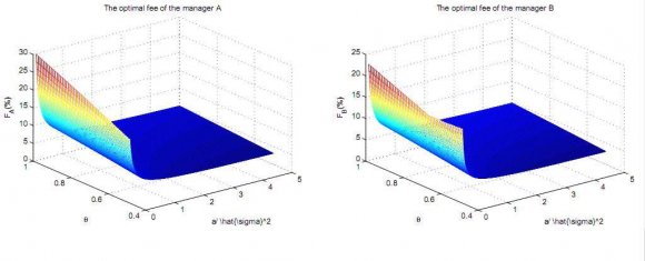
![3) b) The CPT Risk Criterion Before we define the value function and the objective function of a CPT-investor, we introduce two indispensable and classical definitions. Global Journal of Management and Business Research Volume XIX Issue V Version I Year 2019 ( ) C Dynamic Money Doctors under Cumulative Prospect Theory Definition When investor i chooses manager j to invest wealth in the risky asset, if ? i is uniformly distributed on [1 ? ?, 1], we definite the value function of a CPT investor as follows:](https://journalofbusiness.org/index.php/GJMBR/article/download/2817/version/101764/1-Dynamic-Money-Doctors_html/25990/image-3.png)
| Year 2019 |
| 8 |
| Volume XIX Issue V Version I |
| ( ) |
| Global Journal of Management and Business Research |
| © 2019 Global Journals 1 |
| Year 2019 |
| Volume XIX Issue V Version I |
| ( ) |
| Global Journal of Management and Business Research |
| Dynamic Money Doctors under Cumulative Prospect Theory | |||||
| when W i,t ? 0, it is easy to show that | |||||
| max V i,t | U (W | T i,t , f j ) | |||
| a? i,j ? 2 = ( = ( a? i,j ? 2 ? f j ) ? W ? i,t max k i,t ?0 | G i,t (k i,t ) | ||||
| Year 2019 | = ( Similarly, when W i,t < 0, we get that a? i,j ? 2 ? f j ) ? W ? i,t A i,t . | (8.14) | |||
| 22 | max V i,t | U (W | T i,t , f j ) | ||
| Volume XIX Issue V Version I | = ( = ( Therefore, | a? i,j ? ki,t <0 a? i,j ? (8.15) L i,t ( ki,t ) | |||
| ( ) C | max V i,t | U (W | |||
| Global Journal of Management and Business Research | |||||
| © 2019 Global Journals 1 | |||||