1. Introduction
ublic transport occupancy is a very important indicator. On the one hand, low occupancy rates result in a low payback of transportation. On the other hand, too high occupancy rates reduce the quality of services provided to passengers, which can lead to an outflow of passengers.
The study of occupancy of public transport devoted some works. In [1], the authors found that Pareto law is valid for many routes about occupancyonly 20% of bus occupancy is used for 80% of the route. The article [2] presents a method for estimating the level of employment of public transport based on data recorded by the weighing system in motion (wait in motion system). Analysis of the measurement data allowed us to propose the following analytical form of a function describing the employment level of a passenger vehicle, depending on the result of gross weight measurement [2, p. Five]: Y = 152.05X + 9624.4, Where X is the number of passengers, Y is the vehicle weight.
The coefficient of determination for this expression is 0.79. The values of the remaining statistical criteria, the authors do not give. It should be noted that the method proposed by the authors allows you to quickly and accurately determine the number of passengers transported on the stretch. At the same time, such installations are quite expensive. Also, with their help, it is almost impossible to assess the change in occupancy op the length of the route, especially in one day to conduct complete surveys of passenger traffic.
In work [3] the information about the dynamics of changes in the occupancy of buses of the EU countries is given. The authors emphasize that the level of employment for buses varies between the Member States. For example, in the UK, the bus transports an average of about nine people, while in France this figure is about 25. The authors explain the differences between member states by different public transport organizations (tariffs, frequency, availability, etc.), as well as ownership of bus companies. Similar studies for the United States are given in [4].
The purpose of the work is to calculate and analyze the statistical characteristics of a random variable characterizing the degree of utilization of the capacity of trolleybuses in the city of Mogilev. The degree of capacity utilization is supposed to be evaluated by the following criteria: ? Average occupancy per flight (Nr), equal to the ratio of passenger-kilometers made for the trip to the length of the trip; ? The coefficient of trip capacity (Krvm), the value of which is equal to the ratio of passenger-kilometers of transport work performed during a journey, to the maximum possible transport work, determined by the product of the capacity of the trolleybus by the distance of the trip; ? Passenger density factor (Kp), the value of which is equal to the ratio of the maximum passenger traffic per flight (passenger density) to the capacity of the trolleybus; Bus, trolleybus, and electric bus traffic, as well as route taxis, are organized in Mogilev. In the city there are Branch "Bus depot No. 1 of Mogilyov", Branch "Automobile park No. 22 of Mogilyov", Branch "Automotive park No. 3 of Mogilyov". The trolleybus traffic in Mogilev was opened on January 19, 1970, and has six routes (Figure 1). The operating organization is OJSC "Mogilyovoblavtotrans", which includes one trolleybus park. From February 2018, two electric CRRC TEG6125BEV03 electric buses began to run in Mogilev along the trolleybus route No. 4.
To calculate the three above criteria for characterizing the degree of utilization of the capacity of trolleybuses, a selective survey of passenger traffic was carried out on each route. It was done by direct observer counting the number of incoming and outgoing passengers at each stop. The total number of flights surveyed is 110. Statistical characteristics of the studied criteria are presented in Table 1. Evaluation of descriptive statistics shows that the mean and median are not significantly different from each other. This is an indirect sign that the distribution of the random variables under investigation is subject to the normal (Gaussian) distribution. However, the difference between the Skewness modulus and the standard Skewness error is more than three times, the difference between the kurtosis and the kurtosis error is also more than three times. This is an indirect sign that the distribution of the random variables under study is different from the normal (Gaussian) distribution. Figure 2 shows the distribution diagram of the random variable under investigation and the corresponding statistical tests.
The Study of the Trolley Buses Occupancy From the constructed histograms it can be seen that their shape is visually different from the theoretical curve of the normal distribution. This is a sign that the variables are different from the normal (Gaussian) distribution. The level of significance for the Kolmogorov-Smirnov test is more than 0.2 for Np and Krvm. This indicates the normal distribution of a random variable. The level of significance for the Kolmogorov-Smirnov test is less than 0.2 for Kp. This is a sign that the variables are distributed according to a distribution other than normal(Gaussian). At the same time, the significance level for the Shapiro-Wilks test is less than 0.05 for all three random variables under study. This is a sign that the distribution law of the quantities studied is different from the normal (Gaussian) distribution. Figure 3 shows the normal-probability graphs of the distribution of random variables under study. From figure 3 it can be seen that for all three random variables under study, the actual data have some variation relative to the theoretical straight line. This indicates that the random variables under study are different from the normal distribution. Figure 4 shows the box scatter diagrams of the random studying variables. From figure 4 it can be seen that the diagrams are asymmetric concerning the median, and there are outliers and extreme points. This indicates that the random variables under study are different from the normal distribution.
Thus, by the studies performed, it can be argued that the distribution of average occupancy per flight (Np), coefficient of voyage capacity (Krvm) and coefficient of passenger density (Kp) is different from normal(Gaussian) distribution.
The results of fitting the distribution in the Statistica program showed for the three random variables studied using the p-values of the Kolmogorov-Smirnov, Anderson-Darling and Chi-square tests are shown in Table 2.
2. Rayleigh distribution
The Study of the Trolley Buses Occupancy
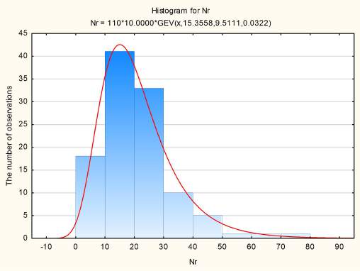
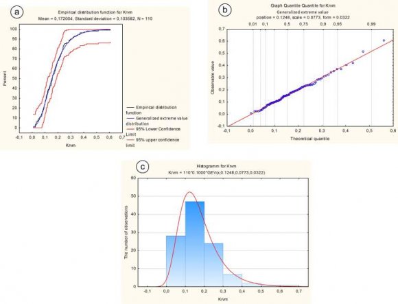
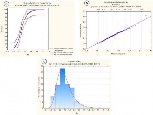
Figure 5 shows the graphs of the empirical distribution functions and the quantile-quantile graphs of average occupancy per flight (Nr). From figure 5 it can be seen that both graphs show that the Generalized extreme value distribution is the best fit to the observed data for the variable Nr. The corresponding distribution histogram is shown in Figure 6. Similar actions were performed for the remaining variables. It was found that the best fit for the variable Krvm is the Generalized extreme value distribution (Figure 7), and for the variable Kp -the Johnson's SU-distribution (Figure 8). For a sample size greater than 30 values, by the central limit theorem, the required sample size n for estimating the mean, in cases where the variance of the entire set is not specified, can be found using the following formula [5, p. 197 ? The coefficient of regular capacity (Krvm) provides the maximum absolute error of this random variable of 0.02%; ? The coefficient of passenger density (Kp) provides the maximum absolute error of this random value is also 0.02%.
So it can be argued that in the city of Mogilev when passengers are transported by trolley buses with a confidence level ? = 0.95, the mean value:
1. Average occupancy per flight (Nr) is 21 passengers with the maximum absolute error of three passengers. 2. Average coefficient of trip capacity (Krvm) is 17.2% with an absolute error of 0.02%. 3. Average passenger capacity ratio (Kp) is 30% with a maximum absolute error of 0.02%.
Further research should be directed to:
? A comparative analysis of the degree of occupancy of public transport in different countries and testing the hypothesis that the degree of occupancy of buses is influenced by macroeconomic indicators in the country: GDP per capita, foreign trade balance, etc. ? Check the differences in the criteria for assessing the degree of capacity by route, by the hour of the day. ? Search for the relationship between bus occupancy, route characteristics and transportation payback; ? Development of measures to optimize the degree of capacity utilization.
| Random value | Average Median | Standard deviation | Standard error | Skewness Standard error of skewness Kurtosis | Standard error of Kurtosis | ||
| Nr | 21,15643 19,20375 12,74059 1,214768 1,275671 | 0,230448 | 2,735502 | 0,457021 | |||
| Krvm | 0,17200 0,15613 0,10358 0,009876 1,275671 | 0,230448 | 2,735502 | 0,457021 | |||
| Kp | 0,29956 0,27642 0,16564 0,015793 1,225317 | 0,230448 | 3,127494 | 0,457021 | |||
| Distribution law | |||
| Kolmogorov-Smirnovtest | Anderson-Darling test | Chisquare test | |
| Average occupancy per flight (Nr) Generalized extreme | Generalized extreme | Mixture distribution | |
| value distribution | value distribution | ||
| Ratioofcapacity (Krvm) | Generalized extreme | Generalized extreme | Weibull distribution |
| value distribution | value distribution | ||
| Coefficient of passenger density | Johnson's SU-distribution Generalized extreme | ||
| (Kp) | value distribution | ||
| 0,195 12, 74059 2, 48 ? = ? = . That is, a sample of 110 | ||||||
| values of average occupancy per flight (Nr) provides the | ||||||
| maximum absolute error of 2.48 passengers. | ||||||
| Performing similar calculations can be obtained that 110 | ||||||
| values: | ||||||
| Where ? -marginal relative error; | ||||||
| ? -maximum absolute error; | ||||||
| x -sample mean; | ||||||
| t? -Student's ?-quantile distribution with n degrees of | ||||||
| freedom; | ||||||
| x ? ? = = | t s x n ? | (1) | s -sample standard deviation estimate. | |||
| By value | x ? ? = = | 0, 2 = = and 12, 74059 0, 6022 21,15643 s x | (see table 1) we get: | |||
| 0, 2 = | t ? n | 0, 6022 | t ? n ? = | 0,3321 | (2) | |
| From the table of values confidence level ? = 0,95 (technical sciences) and t ? n [5, p. 197], at 0,3321 t n ? = it can be obtained that a sufficient sample size for estimating the average value of the | average occupancy per flight (Nr) is 37. Knowing that the sample size is 110 values and ? = 0,95 from the t ? table of values n [5, p. 197], can get that 0,195 t ? = n . Then from expression [1),] you can get | |||||