1. Introduction
Hen Gompertz(1825) formulated his "universal mortality", which later became famous, he could not have imagined that it would have become an important tool to measure the aging process, not only of the human population, but also for experimental applications in species of animals and, more generally, in the bio-demographic approach to mortality modelling (Kirkwood, 2015).
2. law of human
In time,other models were introduced although the Gompertz model never lost its luster because it continued to play an important role in the development of theoretical hypotheses in relation to the patterns of mortality at old ages. This method has connections to the evolutionary theory of senescence (Rose, 1991;Tuljapurkar, 1997;Ricklefs and Scheuerlein, 2002) and examines the increase in mortality hazard at older ages because of differential increased physiological vulnerability due to environmental conditions during preadult ages. This process is referred to as "actuarial senescence" or "actuarial aging" and the actuarial method supplies the so-called aging measures; these are obtained, among others, through the parameters of the model used to describe the course of actuarial senescence.
Within this framework, the present paper studies the actuarial method for life table analysis. The results can be different depending on the approach used to study the phenomenon: A period or a cohort approach. In the first case the level of mortality is influenced by the conditions "of the moment", whilst the second case brings to light the long-lasting effects of living conditions experienced from pre-adult age.
It is exactly on these latter aspects that this work focuses by examining a particular period in Italian history. It is a critical examination of both the approach and the explanation of the results provided by the actuarial method for life table analysis by cohorts and regards the mortality of young Italian adults who experienced the impact of World War I (W W I). This applies both to the soldiers who fought on the war front and to the women who remained at home or at work and suffered hardships.
"rates of aging" that are used to describe actuarial II.
3. Materials and Methods
the elderly population in Italy has found a more robust database than in the past because the demographic change was characterised by an intense process of population aging that began with a rapid decline in fertility and an accelerated reduction in mortality.As a result, there has been a steady increase of the elderly (Preston et al., 1989). According to a recent study (Bonarini, 2009), in Italy the census of 1971 revealed that there was already a considerable number of centenarian women and this number increased progressively with the generations born after 1881 there is also the HMD source, but its data regarding the period of interest for the present study presents a lower quality for the period 1872-1905, as HMD (2015) clearly specifies. Therefore, the HMD source will not be used directly, because that work could lead to consider also the differential mortality by gender at old ages, which is a subject that has already been studied (Maccheroni, 2014) using Istat period life tables. As a consequence, the comparisons of the results obtained from period life tables and birth cohort-related life tables refer to the same source. 2 is possible to get enough data from the population to construct the probability of death and period life tables for those aged over 100; this especially applies to the 1970s and 1980s. There are, however, graduation methods (Thatcher, Kannisto, Vaupel, 1998) which enable to extrapolate the probability of death for the age ; on the other hand, the number of centenarian men grew at a much slower pace. economy in order to support those who were at the warfront. In the Appendix there is a brief historical digression that may help to focus on this aspect (also see the relevant bibliography: Schaumann, 1993). The birth-cohorts studied here are those born during the period from 1889 to1919. This choice is obviously conditioned by the statistical data available (Istat, 2002) that does not give a complete picture of the mortality rates of all the male cohorts engaged in the conflict. Nevertheless, out of the cohorts examined, those that were born between 1889 and 1899 are the ones who suffered the experience of war to a much greater extent.
In recent years, the mortality analysis of extinct cohorts of W W I veterans born after 1889 was based on death probabilities that in Italy Istat 1 has provided since 1974 in the time series of period life tables. As is known, which has so far built only period life tables, followed this approach to determine the probabilities of death at elderly ages. Presently this Institute provides the homogeneous 1974-2014 time series where period life tables end at age 119 (demo.istat.it);obviously, this ultimate age is older than the oldest age in the population. In the birth cohorts tables that have been rewritten starting from the previous ones, the ultimate age considered is the one after which the number of survivors in the table is less than 1.The ultimate age for men is 108 3 years up to the 1900-birth cohort, and 109 years for the following cohorts. Conversely, women ultimate age is 109 years up to the 1892 birth cohort, and 110 years for the following cohorts (Kannisto, 1994). As already specified, the actuarial aging study affected cohorts born from 1889 until 1906, already extinct in 2014. Hence, all the related probabilities of death were obtained by processing Istat 1974-2013 time series. The aim of this work is also, however, to understand the effects of the war and of the Spanish flu on cohorts born in those years and to compare these results with them of cohorts born during the years preceding those events. It is for this reason that the life tables of cohorts born between 1907 and 1919 were closed with an extrapolation made according to the Gompertz model For several years, the study of mortality among Despite this, it is not advisable to assume that it group for which the available data are uncertain. Istat, [1] since those cohorts were not yet extinct in 2014.
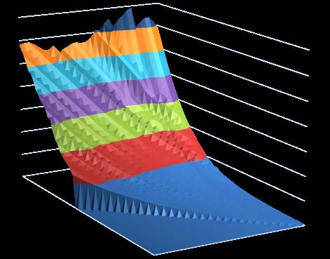
As a first step, the Gompertz model was fitted to mortality data from age 85 onwards (Vaupel et al ., 1998) in order to study the actuarial aging for cohorts born between 1889 and 1906, and some very satisfying results were obtained (see R 2 in table 1, following paragraph). It is precisely from these results that one proceeds to adapt and to extrapolate the [1] to the following cohorts, which leads to conclude the birth cohort life table with a minimal addition for the 1907 cohort and with consistently greater integrations for the others, up to and including the 1919 cohort. Our reconstruction of the extinction process of all the considered birth cohorts are shown in figure 1,in which the profile of the varying probabilities of death according to age and cohort highlights a general and progressive decline. There were also, however, certain years in which the health of the elderly suffered particularly. Reference is made here, in addition to what happened in 1983, especially to the consequences of the hot summer of 2003 that led in both cases to a net increase in mortality from diseases connected with the circulatory and respiratory systems (Istat, 2011). In figure 1, the effects of these changes are visible beginning with those born in 1919 and aged 84 and continuing up to those born in 1904 and aged 99.
Figure 2 gives us a preview of some of the results under study in the following paragraphs. Here it is evident that those who were born during the war experienced a much higher old age mortality than those who were born immediately before or after this period. In fact, the rise in the mortality profile for both males and females clearly show this phenomenon, known as the cohort effect.Moreover these findings suggest that the regarding females: it relates to the generations born between 1892 and 1897; these women were young adults during the war and they probably suffered more than men did from the very poor living conditions, which may have led to poor health status in later life. Fig. 2: Cohort probabilities of death within a five-year period ( 5 q x ) at selected ages, by gender and year of birth mortality ( 5 q x ) decreases quickly for both genders and in particular for women. Fig. 2 also gives evidence of a "selection" effect in the case of 90 and 95-year-old survivors, because in these cases the effect of severe living conditions throughout the war period is not visible for the cohort mortality born between 1889 and 1900. As mentioned, in Italy the present day aging of the population is caused not only by the decline of fertility, but it is also part of a profound change in the death rates at advanced ages (Vaupel, 2010) whose trajectories have for many years been characterised by a continual decline in pace. Obviously it was not so in the past. Between 1960 and 1980, life expectancy at age 60 for men remained stationary, whilst life expectancy for 80 year olds even slightly decreased between 1970 and 1980. It is during this period that the birth cohorts that in youth or adulthood experienced the wartime conditions with its uncertainty, suffering and deprivation, either died out or reached very advanced ages. In order to focus on their mortality, the Gompertz one, not considered here because it implies, amongst other notions, that the causes of death of young adults and of the elderly are independent. The Weibull model also describes better the mortality for purer, single causes-of-death, while the Gompertz model is better for describing 'all-causes' of deaths (Juckett, Rosenberg, 1993;Gavrilov, Gavrilova, 2001). mortality (Pollard and Valkovics, 1992 The effect of the end of W W I emerges for people who in those years were on the threshold of adulthood -those born between 1898 and 1902 -and who therefore experienced more rapid decline in mortality than the cohorts born before. At age 85 the Spanish flu epidemic didn't influence the survival in later life of those who were born at the end of the war. There is a similar "hump" in the 5 q 85 profile (fig. 2), particularly model 4 was chosen from among the available models as it has been widely employed to represent senescent 4 Another model employed for studying actuarial aging is the Weibull and it takes into account the legacy of living conditions in youth and adult ages as illustrated below.
The model (Kirkwood, 2015) describes the increase of the mortality hazard, expressed by the increasing age x; it results in a mortality trajectory that reflects the increasing vulnerability of individuals because of declining physiological functions with aging. The formalisation of Gompertz's hypothesis about instantaneous rates leads to the following expression for the force of mortality ?(x) = ? a exp( ?x) [1] For a long time evolutionary biology has studied the questions of why senescence occurs and Gompertz therefore represents one of the fathers of this discipline because with his model he went beyond the empirical observations about patterns of mortality in order to attribute biological significance to life tables. Between this discipline and the evolutionary theory of senescence there are obviously large intersections; the latter proposes, among other things, a substantial partition of total mortality in extrinsic and intrinsic (Carnes and Olshansky, 1997;Carnes et al., 2006); this partition does not claim to be exhaustive but to support the experimental analysis. The former, being the consequence of external or violent causes, is ageindependent and accounts for most pre-adult mortality; the latter is age-dependent. At the origin of extrinsic mortality there are, in fact, external causes such as environmental disasters, famine, severe climatic conditions and war, as in the case considered. Instead, physiological functions of an individual.
For both disciplines here cited, the Gompertz model [1] thus incorporates the two components of mortality with these two parameters: the extrinsic one with ? a ? typical of the pre-adult or young adult ages ? and the intrinsic one with ?, the expression, at advanced suggested the idea that early life experiences have an impact on health and mortality in later life (Kuh and Davey Smith, 1993).
The real significance of the word "early" in those contexts is not exactly the same for all the authors.Consequently, this approach presents a margin of arbitrariness from an applicative point of view: on the one hand ? a is defined as an age-independent term, on the other hand, when [1] is adapted starting from the adult age, ? a is associated with extrinsic mortality. In the vary from society to society and may change over time, with the results of a mathematical model that describes the relationship between "chronological" age and mortality rates within an age group, whose threshold is still conventional.The estimates of the parameters for the same cohort will therefore vary depending on the age groups to which the model fits.
Broadly speaking IMR is a scale or level members of all cohorts at all ages and then raising or lowering the mortality curve. Depending on the case, this level of mortality can be associated with hazard present in the history of the entire cohort, which in the present case is actually observed.
To fit [1] to the cohort life tables, the probabilities of death q x (fig. 1) were converted into instantaneous rates of mortality ? x , which can be conveniently approximated as
? x ?-ln(1-q x )The parameter estimates of ? a and ? were estimation method based on the log-arithmetically transformation of ? x ; as mentioned in the previous paragraph, the results of the adaptation have been very satisfying as can be observed by the index R 2 (tab. 1).
instantaneous rate or the force of mortality ?(x), by where ? a and ? are constant. The first is also known as initial mortality rate (IMR) (Finchet al., 1990) and a is the age starting from which ?(x) grows exponentially; the second,i.e.the mortality increase rate, describes how intrinsic mortality is the result of the decline of the ages, of vulnerability that is also the legacy of the past.
Hence, [1] implies that the increase in mortality rate by increasing age represents increasing vulnerability due to external causes suffered by young adults.On this point, it is worth considering that epidemiologists too parameter or background mortality rate affecting every obtained through the software STATA byusing the OLS latter case, references to social age concepts such as adulthood or old age could be reconciled; these may this vulnerability increases by increasing age.
Equation [1] should therefore apply starting from early adult life, but for more recent cohorts it generally best fits data pertaining to the over 80's. In order to graphically represent [1] from an arithmetic point of view,a transformation of ?(x) is used and, as such, ln ?(x) appears as a straight line by increasing x; ln ? a is its intercepts and ? is its slope: this is the term with which ? is often indicated.
4. Results and Discussion
Even though these analyses focus on mortality from age 85 onwards, rather than adult ages onwards, parameter estimates may have a preliminary interpretation according to the evolutionary approach, especially evident as far as men are concerned.
With regard to IMR estimates, and apart from the mortality level that they provided, IMR shows, comparatively, the highest values for those born until 1897 (tab. 2), thus registering a high mortality that may be linked to the hardships of the wartime. As a matter of fact, from a comparison with cohorts born after 1900, for declining (tab. 1), it can be deduced that with the passing of time the long-lasting deleterious effects of war on cohorts with range of birth dates from 1889 to 1899 did not disappear.
The IMR model-based estimates show, obviously, lower levels for women than for men, although the strong correlation among genders (Pearson's r = 0.929) confirms the harshness of the wartime living conditions for civilians, in particular for the In addition, the slope time series regarding male and female are highly correlated with each other (r = 0.958). Actually for female birth cohorts born after 1897 and for male ones born after 1898 (tab. 2 and fig. 3 The comparison between IMR -the background mortality rate -and slope estimates is in line with the These cases were already known as Strehler and Mildvan (1960) used for the construction of two indexes both indicatedas "rates of aging" (Ricklefsand Scheuerlein, 2002) or aging measures, which are independent from age. One of these indexes is known as mortality rate doubling time (MRDT) and it is a ? transformation [2], the other one is the so-called ? index.
The parameters of the Gompertz model [1] are which the estimates are much lower and IMR steadily younger ones. As in the case of their male peers, similarly for women the highest values of IMR are in fact those of cohorts born during the 1889-1897 period.This aspect will be analysed later on. B) there is a turning point, after which the slope increases faster. However, this is not related to the cohorts born 1898 onwards -especially for women ? the level of mortality, ? 85 (?) [4], decreases quickly, as can be observed in fig. 3 E Let us examine the first, This index indicates after how many years the risk of death tends to double. In human populations MRDT usually should be included between 7 and 8.5 years (Finch et al., 1990), which respectively identify a situation of low and high mortality (Gurven and Fenelon, 2009).Unfortunately, this statement is not correct because low or high mortality depends on mortality rates, even if there could be a relationship between an aging measure [2] and a summary index of mortality [4],
As shown in fig. 3 C and in tab. 1, there are some important differences between genders.
In the case of males, cohorts born between 1889 and 1898 show MRDT values slightly above 9: they are the generations that were between 17 and 26 years of age at the beginning of the war. The MRDT trajectory declines slowly until the 1897 birth cohort, then the decrease stops up to the cohort born in 1898. The 1897-1899 cohorts were sent one after other to the war front in the most dramatic period of the conflict, after which the successive generations experienced a gradual reduction in actuarial aging. as will be seen later on.
5. MRDT = ln 2 ??
As regards females, MRDT values are all within those of the previous range -i.e. between 7 and 8.5 years -but the index grows after an initial decrease, it reaches its maximum precisely with the cohort born in 1897, and then it starts to decrease again (fig. 3-C). This trend highlights the important contribution offered by women in all fields: they, as all those who were not on the war front, had to substitute men in all jobs and activities. The cohorts of men born between 1874 and 1900 were gradually called to arms, even though only the youngest were involved in military operations. About five million men thus left their productive work, which is why women were called to fill up the resultant vacancies, mostly in farming and factories. They too were subject to food rationing and experienced a decrease in their purchasing power due to the taxation levied to finance the war. They were deprived of health care because almost all the medical staff was concentrated at the war front.
Thinking of wartime, one usually thinks of soldiers, their courage, their struggles, their hard conditions and pains, but seldom thinks of women, who were strongly involved in war too and experienced all hardships, thus feeling the effects of war tragedies.
It should also be noted that the Italians' living conditions had already worsened previously, because the war started in Europe the year before had had serious repercussions on the economy even in the other non-belligerent countries. Moreover, to make things still worse, a devastating earthquake had hit a wide area of central Italy in January 1915.
The years following the war were hard too and the period life tables highlighted an increase in female mortality at puberty age (Pinnelli, Mancini, 1997), the cause for which lies in their low standard of living. The other index isthe so-called?index [3] which is a geometric mean between two rates and hence it is a rate itself.
The results of [3] are also in line with expectations and their trajectories present a profile, which is very similar to MRDT (figures 3 C and 3 D).
Nevertheless,for a comparative analysis between these two measures of the rate of aging it is necessary to consider that they are strongly correlated with the parameters of model [1]: more particularly tab. 3 reveals that, for both males and females, the Pearson correlation between ? a and ? is practically 1, and it is almost 1between ? a and MRDT. On the contrary, ? with ?, and ? with MRDT, are strongly negatively correlated with each other (tab. 3). Actually, if both measures show that the substantial actuarial aging decrease begins with the cohort born in 1898, the MRDT decline between 1897 and 1906 is only 12.7% for males and 16.7% for females, whilst decreases of 39.8% and 52% are obtained from ?, which are over three times higher. There are therefore two very different measures of the changes in the rates of the actuarial senescence, which is difficult to be explained as it regards just ?, unless one refers to its relation with ? a , whose decrease in that period was also very substantial: 68.3% and 80.8% respectively for males and females. Let us examine the relation between ? a and ?.
By construction, ? is the geometrical mean between ? and ? a [3]; in the present case, ? a is always smaller than ? (tab. 2). If one denotes by ?* the arithmetical mean between ? and ? a , according to the properties of the means (Hardy, Littlewood, Polya, 1964), the following relation is worth
? a <?<?*<?Consequently, ? a has the greater weight on ? and the strong relationship between ? a and ?indirectly confirms this fact (tab. 3). This result gives rise to doubts as to whether ? can be used as the rate of relative aging in the age group here considered.
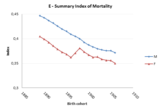
Instead, the variation in the MRDT level depends on the ? trajectory that increases with the decrease in mortality (Hawkes et al., 2011); the use of a summary index of mortality confirms that. The chosen index was proposed by Schoen (1970) who recommended the geometric mean of the age-specific mortality rates as a summary index of considerable ? = ?? a ? [4] where x max is the last age and i = 85, 86 ? (x max -1). Indeed,as our analyses show (tab. 3), the relationship between ? and ? 85 (?) is negative for males (r = -0.88 ), whereas for women this inverse relationship is evident from the birth cohort 1898 onward (r = -0.687), where their mortality levels began to decline continuously. Fig. 3 A and fig. 3 E show the association of ? 85 (?) with the values of background mortality (? a ), which is very strong in the case of males (r = 0.968 ), less strong in the case of females (r = 0.727). This happens also because the aging-related mortality in the Gompertz model [1] increases exponentially as a multiple of ? a .
A review of the previous findings concludes by crossing them with those of the perhaps best known indicator of the mortality level which is precisely the birth a) Mean lifetime in cohorts born between 1889 and 1906
As already stated, these birth cohorts completely died out and the relative life tables were of women whose temporal sequences of aging measures are characterised by two phases is especially evident in figures 3 C and 3 D.In the first, an initial slight decrease of ? and MRDT is followed by a sharp turnaround in tendency between the birth cohorts of 1894 and 1897, when the actuarial aging reaches its maximum.The second phase is characterised by a continued sharp decrease of the indexes. In the case of males, there is only one break in the trend of decrease, always circumscribed around the generation born in 1897. Again,as to women, ? 85 (?) shows an increase in mortality for birth cohorts from 1896 to 1898 too The legacy of war is also evident from the Fig. 4: Average number of years actually lived after 85 from birth cohorts and corresponding remaining life expectancy of fictitious cohorts at the same ages. Italy, males and females One of the most recent studies (Rogers et al., 2010) shows that the lower incidence of cardiovascular diseases in women, with consequent lower mortality, is due to the positive action of female sexual hormones on blood fat levels.However, this protection ceases after menopause and hence social and environmental factors, in particular the family, educational and working environments, determine the mortality differences at all ages, also indicated as main causes (Maccheroni, 2014). The study of women's life paths who reached these ages led to identify a further explanation of higher longevity in women: their psychology, which leads them to build social and solidarity networks in a much more efficient way than men do. Thanks to their different way of relating to the external world, women show a higher capacity to adapt to life's changes, to life's various cohorts average length of life; it is here indicated by e 85c to distinguish it from e 85p which is the corresponding period life expectancy. We begin with a comparison of the aging measures, which concern only cohorts born between 1889 and 1906; however, as regards the average length of life the analysis covers a longer time span.
reconstructed entirely based on Istat database.The case there are no signs of these reversals in the trend of the mean life span, but only a gradual slowing down (fig. 4) after an initial growth, precisely for cohorts born from 1894 to 1897. However, the remaining lifetime increased slowly: from one generation to another with respect to those born between 1889 and 1906, the average increase is approximately fifteen days for both genders.
comparison between the evolution of e 85c and e 85p . Fig. 4 shows that the cohort effect was lower for those born up to 1897 with respect to those born afterwards: their e 85c was slightly higher than the corresponding e 85p by approximately one month and a half both for males and females. Conversely, for those born after 1897 the increases were much higher, especially for women. The latter in fact benefited more during the last few years of their existence from the progress made in living conditions since the early 80s, both with respect to the past and with respect to the men, as shown by the gap with the corresponding period life expectancy (fig. 4). Consequently, the gap between mean residual lifetimes increased tending to be higher than that which emerges from the comparison of life expectancies.
? 85 (?) = ( x max -86 )
? ? i ? i 85 <x <x max (fig. 3 E), but it has only a little effect on e 85c . Indeed
IV. A Demographic Focus on Mortality Rates: Mean Remaining Lifetime After Age 85 stages and to changing human relationships (Cesa Bianchi, 2000). In order to carry out an analysis of mortality for the cohorts whose range of birth dates 1907-1919, it was necessary to close the related life tables by extrapolating a logarithmic transformation of [1] at late ages. This is because the high values of the R 2 suggest that also in their case the regression model fits well, and they validate its use for predictive or forecasting purposes.
The results display another consequence of the common: e 85c of individuals born between 1915 and 1918 shows a severe decrease which reaches its minimum with the birth cohort of 1916; thereafter only with respect to those who were born after 1917 does the decrease lessen rapidly (fig. 4). It might also be observed that men belonging to these cohorts took part in World War II in pre-adulthood, so that even in their case the consequences of that event could affect their mortality at older ages.However, the perfect synchronism that characterises the e 85c trajectories for consequences greatly. The bases of these findings are to be linked to the rise in mortality in the extreme age groups that had already been disclosed by the temporal sequences of the probabilities of death given in fig. 2. It is only for the individuals born in 1919 that the average length of life realigns itself on the temporal trend prior to the beginning of the war. This occurs even though about half of those born during the widespread Spanish flu epidemic which, in Italy in its acute phase, raged between autumn 1918 and early summer 1919 5 b) Mean life time in cohorts born between 1907 and 1919 ; according to the chronicles, in its early phase the epidemic struck above all the soldiers on the front before spreading nationwide (Melegaro and Alfani, 2010). These latest findings indicate how a sudden and adverse change in the living and environmental conditions experienced at the time of birth of these generations can have negative repercussions on their mean remaining lifetime (Barker, 1994) even at older ages. Moreover the increase in infant mortality during the years of the conflict, which ceases precisely in 1919, as illustrated in tab. 4, provides a further element of proof, albeit indirectly, of the deterioration of living conditions.
war that both living male and female groups have in both males and females (fig. 4 It should however be noted that, in the past, there had been other cases in which the adverse environmental conditions did not lead to what has now been highlighted in relation to the war in 1915-1918. A comparison of almost the same ages can be done with the results of a study of cohorts born in Finland during out that their mean remaining lifetime at 80 years of age was not less than that of birth cohorts born either five years before or five years after the famine (Kannisto, Christensen, Vaupel, 1997). In the case under study, the war situation and related family and social interactions affected pregnant mothers and those with very young children.These found themselves alone whilst their husbands were on the front, in a different way from experiencing this different cohort effect on later life mortality (fig. 2).
In the case examined, statistics alone do not allow for speculation on why pregnancies during the war and the conditions under which the births took place in Italy had such drastic effects on long-term health and hence on mean remaining lifetime of these cohorts (Elo, Preston, 1992).
V.
6. Conclusions
The Gompertzian aging model provided a good fit to the mortality rates of the birth cohorts that have herewith been examined, thus making it possible to perform a comparative analysis of both the role assigned to the parameters and of the aging measures ( [2] and [3]) proposed by the actuarial aging or senescence.
The evolution of the model-based estimates of parameter ? a clearly highlights that for cohorts born between 1889 and 1900, on the threshold of 85, the negative legacy of environmental conditions determined negative effects affected, albeit in a different selective way, both males and females. On the contrary, for those improvement in their living standards, the background mortality saw a steady decline, that resulted in a decrease of rates of senescence.Hence it appears that the well-known William's hypothesis (1957) -according to which "low adult death rates should be associated with low rates of senescence, and high adult death rates should be associated with high rates of senescence" 6 therapies introduced by biotechnology and progress in molecular nanotechnology and artificial intelligence ( is supported also in this case (tab. 1).
Yet, it should be noted that demographic analyses revealed that the Gompertzian pattern is valid only for a part of the human life course. Recent studies have shown that human mortality rates do not continue to accelerate at very advanced ages, but rather decelerate (Vaupel et al. 2010), thus contradicting equation [1], where the slope quantifies the constant age-dependent acceleration of the mortality rate.
Moreover, from findings provided by the aging measures across the birth cohorts, some critical issues emerge that influence negatively the heuristic component of this type of research, when referred to human mortality.
The trajectories of ? and MRDT concerning cohorts born after 1899 highlight two different reductions of actuarial aging that ? amplifies significantly; so one The question is whether today extrinsic mortality still plays a role in driving the evolution of aging in societies with low-mortality rates, also because of the difficulty to distinguish clearly between "external" and "intrinsic" forces that influence vital rates. The social environment strongly affects human lifespan: the improvements in medical care, the prevention of major death causing diseases and changes in life-style have minimised both the infant and the pre-adult age mortality rate, which is almost exclusively extrinsic and above all caused by road accidents. At advanced ages, one far-reaching consequence was the deceleration of the process of deterioration by increasing age and the related mortality postponing (Vaupel et al., 2010) that involved a distinction among early, middle and late old age too. www.a4minfo.net) will not stop the aging process, but it could however lead to a reassessment of old age with respect to how it is currently considered. These interventions are at the origin of the biological processes cannot say which measure is better because there are nocriteria for choosing between them.
7. born after 1900 who experienced remarkable
The combination of medical research, new Another great revolution is taking place in our societies, whose objective is not an increasing longevity but rather a longevity without disabilities and functional dependence.
the great famine of 1866-1868. Here the findings pointed those who lived during the famine in Finland, thus by the war had not been cancelled out still. Such of the "natural" deteriorating of the physiological functions leaving room for a kind of 'manufactured survival'. Thus, there could be an impact on the mortality pattern at older ages,so the assumptions underlying the application of the models used for the study of the actuarial aging could be undermined.
8. Appendix: A historical outline
In Europe on the eve of World War I two alliances met face-to-face, the Triple Entente (United Kingdom, France and Russia) and the Triple Alliance (Austria-Hungary, Germany and Italy); the latter was of a defensive nature and guaranteed military support to whichever ally came under attack by another State. As is widely known, the conflict began with Austria-Hungary declaring war on Serbia (July, 28 th 1914), which was followed just a few days later by Germany's declaration of war on France and Russia; after that, one declaration of war succeeded another at a frantic pace, thereby ushering in the enormous catastrophe that continued until November 11 th 1918.
Since the expected conditions foreseen by the alliance to intervene in the war were lacking, Italy declared itself neutral, however, it came under strong pressure to support the war effort from two sides. As we know, in the end Italy deployed its troops in favour of France and the United Kingdom. This decision was not only due to the concessions that these two countries guaranteed in the case of victory, but also to a more widespread popular sentiment in favour of these two countries on the one hand, as well as to general sentiments of protest towards the political choice of an alliance with Austria and Germany on the other hand. Moreover, it is necessary to highlight that the birth and building of Italy as a unitary State originated from three wars (1848, 1859 and 1866), known as the Wars of Independence, fought precisely against Austria for the liberation of most of the Italian territories that were then part of the Austro-Hungarian Empire.
Once Italy decided on war in support of France and the United Kingdom, the Italian general headquarters did not proceed immediately with a general mobilisation but rather chose a preliminary individual call to arms to avoid suspicion from the Austrian government. So when the war started on May 24 th 1915 the initial operations were conducted by those who were already enrolled or had been released a short time before, which especially included cohorts born in the years prior to 1895, because in those times all men were conscripted to the army for two years upon reaching twenty years of age.However, besides having recalled the cohorts born in and up to the year 1875, by the autumn of 1916 the army proceeded to bring forward the enrolment of the cohort born in 1897. This
The war initially gave some victories to the Italian army, but early in the fall of 1917, the first phase of the October Revolution gave rise to the conclusion of military operations on the Russian front and this allowed Austria-Hungary and Germany to concentrate their forces on the Western Front. Consequently the Italian army suffered a dramatic defeat (October 1917) at Caporetto and was forced to withdraw to the Piave River.

| Cohorts (males) | ||||||
| 1889 | 1890 | 1891 | 1892 | 1893 | 1894 | |
| ? | 0.073886*** 0.073809*** 0.074235*** 0.074462*** 0.074501*** | 0.074886*** | ||||
| (0.001) | (0.000) | (0.001) | (0.001) | ( 0.001) | (0.001) | |
| ln(? a ) | -7.935739*** -7.937706*** -7.991789*** -8.025734*** -8.043428*** -8.094778*** | |||||
| (0.072) | (0.043) | (0.050) | (0.058) | (0.069) | (0.076) | |
| R 2 | 0.99819 | 0.99874 | 0.99861 | 0.99847 | 0.99825 | 0.99773 |
| Cohorts (males) | ||||||
| 1895 | 1896 | 1897 | 1898 | 1899 | 1900 | |
| ? | 0.075690*** 0.075748*** 0.075774*** 0.075956*** 0.077600*** | 0.078728*** | ||||
| (0.001) | (0.001) | (0.001) | (0.001) | ( 0.001) | (0.001) | |
| ln(? a ) | -8.183682*** -8.203756*** -8.216080*** -8.246453*** -8.423901*** -8.545794*** | |||||
| (0.093) | (0.107) | (0.099) | (0.108) | (0.081) | (0.077) | |
| R 2 | 0.99723 | 0.99682 | 0.99714 | 0.99681 | 0.99772 | 0.99792 |
| Cohorts (males) | ||||||
| 1901 | 1902 | 1903 | 1904 | 1905 | 1906 | |
| ? | 0.079182*** 0.080014*** 0.081084*** 0.083278*** 0.084939*** 0.086772*** | |||||
| (0.001) | (0.001) | (0.001) | (0.002) | ( 0.003) | (0.002) | |
| ln(? a ) | -8.600322*** -8.690346*** -8.798875*** -9.015774*** -9.175651*** -9.365443*** | |||||
| (0.082) | (0.075) | (0.123) | (0.184) | (0.231) | (0.210) | |
| R 2 | 0.99773 | 0.99772 | 0.99605 | 0.99269 | 0.98816 | 0.98644 |
| Cohorts (females) | ||||||
| 1889 | 1890 | 1891 | 1892 | 1893 | 1894 | |
| ? | 0.080707*** 0.080726*** 0.081174*** 0.081539*** 0.081289*** 0.080699*** | |||||
| (0.002) | (0.002) | (0.002) | (0.002) | ( 0.002) | (0.002) | |
| ln(? a ) | -8.693334*** -8.708316*** -8.768037*** -8.821850*** -8.815806*** -8.774603*** | |||||
| (0.187) | (0.165) | (0.183) | (0.209) | ( 0.232) | (0.227) | |
| R 2 | 0.98693 | 0.98880 | 0.98907 | 0.98887 | 0.98874 | 0.98988 |
| Cohorts (females) | ||||||
| 1895 | 1896 | 1897 | 1898 | 1899 | 1900 | |
| ? | 0.080333*** 0.079190*** 0.078718*** 0.079880*** 0.082702*** 0.084639*** | |||||
| (0.002) | (0.002) | (0.002) | (0.001) | ( 0.001) | (0.001) | |
| ln(? a ) | -8.751082*** -8.658132*** -8.627242*** -8.756773*** -9.050620*** -9.254461*** | |||||
| (0.194) | (0.220) | (0.155) | (0.119) | ( 0.114) | (0.101) | |
| R 2 | 0.99232 | 0.99062 | 0.99323 | 0.99439 | 0.99469 | 0.99518 |
| Cohorts (females) | ||||||
| 1901 | 1902 | 1903 | 1904 | 1905 | 1906 | |
| ? | 0.086411*** 0.088008*** 0.088879*** 0.090675*** | 0.092254*** | 0.094545*** | |||
| (0.001) | (0.001) | (0.001) | (0.001) | ( 0.002) | (0.001) | |
| ln(? (0.095) | (0.097) | (0.100) | (0.137) | ( 0.144) | (0.135) | |
| R 2 | 0.99552 | 0.99555 | 0.99588 | 0.99483 | 0.99417 | 0.99358 |
| Cohorts | IMR | Slope | MRDT | ? | ? 85 (?) |
| Males | |||||
| 1889 | 0.000358 | 0.073886 | 9.381255 | 0.005141 | 0.4468 |
| 1890 | 0.000357 | 0.073809 | 9.391080 | 0.005133 | 0.4426 |
| 1891 | 0.000338 | 0.074235 | 9.337164 | 0.005011 | 0.4369 |
| 1892 | 0.000327 | 0.074462 | 9.308800 | 0.004934 | 0.4317 |
| 1893 | 0.000321 | 0.074501 | 9.303914 | 0.004892 | 0.4257 |
| 1894 | 0.000305 | 0.074886 | 9.256069 | 0.004780 | 0.4197 |
| 1895 | 0.000279 | 0.075690 | 9.157736 | 0.004597 | 0.4150 |
| 1896 | 0.000274 | 0.075748 | 9.150663 | 0.004553 | 0.4090 |
| 1897 | 0.000270 | 0.075774 | 9.147560 | 0.004525 | 0.4050 |
| 1898 | 0.000262 | 0.075956 | 9.125617 | 0.004463 | 0.3999 |
| 1899 | 0.000220 | 0.077601 | 8.932251 | 0.004128 | 0.3925 |
| 1900 | 0.000194 | 0.078728 | 8.804351 | 0.003912 | 0.3873 |
| 1901 | 0.000184 | 0.079183 | 8.753793 | 0.003817 | 0.3832 |
| 1902 | 0.000168 | 0.080014 | 8.662780 | 0.003669 | 0.3795 |
| 1903 | 0.000151 | 0.081084 | 8.548518 | 0.003498 | 0.3775 |
| 1904 | 0.000121 | 0.083278 | 8.323303 | 0.003181 | 0.3756 |
| 1905 | 0.000104 | 0.084939 | 8.160558 | 0.002965 | 0.3757 |
| 1906 | 0.000086 | 0.086772 | 7.988134 | 0.002726 | 0.3716 |
| Females | |||||
| 1889 | 0.000168 | 0.080707 | 8.588461 | 0.003679 | 0.4045 |
| 1890 | 0.000165 | 0.080726 | 8.586461 | 0.003652 | 0.3992 |
| 1891 | 0.000156 | 0.081174 | 8.539040 | 0.003554 | 0.3927 |
| 1892 | 0.000147 | 0.081539 | 8.500764 | 0.003468 | 0.3855 |
| 1893 | 0.000148 | 0.081289 | 8.526970 | 0.003473 | 0.3786 |
| 1894 | 0.000155 | 0.080699 | 8.589344 | 0.003532 | 0.3727 |
| 1895 | 0.000158 | 0.080333 | 8.628445 | 0.003566 | 0.3683 |
| 1896 | 0.000174 | 0.079190 | 8.752997 | 0.003709 | 0.3620 |
| 1897 | 0.000179 | 0.078718 | 8.805402 | 0.003755 | 0.3710 |
| 1898 | 0.000157 | 0.079880 | 8.677312 | 0.003546 | 0.3807 |
| 1899 | 0.000117 | 0.082702 | 8.381283 | 0.003115 | 0.3731 |
| 1900 | 0.000096 | 0.084639 | 8.189425 | 0.002846 | 0.3673 |
| 1901 | 0.000079 | 0.086411 | 8.021506 | 0.002617 | 0.3622 |
| 1902 | 0.000067 | 0.088008 | 7.875965 | 0.002429 | 0.3633 |
| 1903 | 0.000061 | 0.088879 | 7.798765 | 0.002332 | 0.3582 |
| 1904 | 0.000051 | 0.090675 | 7.644286 | 0.002156 | 0.3562 |
| 1905 | 0.000044 | 0.092254 | 7.513432 | 0.002010 | 0.3559 |
| 1906 | 0.000034 | 0.094545 | 7.331423 | 0.001804 | 0.3499 |
| Tab. 4: Deaths before age 1 year per 1,000 live births; Italy, 1910-1920 | |||||||||||
| 1910 | 1911 | 1912 | 1913 | 1914 | 1915 | 1916 | 1917 | 1918 | 1919 | 1920 | |
| Males | 146.4 | 162.7 | 135.2 | 145.8 | 137.2 | 153.7 | 174.5 | 159.2 | 194.4 | 134.4 | 132.1 |
| Females | 133.3 | 150.4 | 120.4 | 130.2 | 123.1 | 139.7 | 157.7 | 146.8 | 180.1 | 123.6 | 120.9 |
| ) minimises such | |||||||||||