1. Introduction
rgentina went through several financial crises. According to Kronfelt (2015), the crisis in the early 1930s was due to external factors. Large government deficit and debt were part of the reasons in 3 out of the 4 crises. A real appreciation of the peso and a rigid exchange rate policy were part of the contributing factors in 2 out of the 4 crises. Deregulation of the financial sector, if not managed properly, was another contributing factor. Political turmoil led to uncertainty and dampened economic growth. The 2001/2002 crisis led to bank runs, freeze on bank deposits, default on the $93 billion sovereign debt, the end of the peso-dollar convertibility system, and social unrest.
Argentina continued to display macroeconomic problems including slow economic growth, high interest rates, high inflation, currency depreciation, large amount of government debt, financial account deficits, etc. Real GDP grew only 0.5% in 2014. Monetary policy was unable to provide moderate interest rates and stable prices as evidenced by the relatively high lending rate of 24.01% and inflation rate of 23.9% in 2014 partly due to an increase in M2 by 28% (Ferrandino and Sgro, 2015;Ojede, 2015;Patton, 2015). The value of the peso versus the U.S. dollar declined 47.99% from 5.46 pesos per U.S. dollar in 2013 to 8.08 in 2014 (Pan, 2015). Government debt as a percent of GDP rose from 35.76% in 2011 to 45.28% in 2014 (Edwards, 2015;Georgescu, 2015;Alfaro, 2015). Its financial account showed a huge deficit in 2014 mainly because liabilities were much greater than assets in both foreign portfolio investment and foreign direct investment. International Monetary Fund (2005,2015) provides a review of the Argentine fiscal, monetary and exchange rate policies and presents the issues that need to be improved by the Argentine government.
This paper examines potential impacts of peso depreciation and changes in other relevant business and economic variables on real GDP based on an equilibrium model of aggregate demand and aggregate supply and has several different aspects. First, financial assets are considered in order to take into account the wealth effect. Second, oil prices are considered to determine whether a positive or negative oil price shock would help or hurt the economy. Third, an advanced methodology is employed in empirical work.
2. II.
3. The Model
Suppose that aggregate demand is a function of real disposable income (real GDP minus the government tax), the real interest rate, financial wealth, the real exchange rate, foreign real income or GDP, the real oil price and the inflation rate and that in the augmented aggregate supply function, the inflation rate is determined by the expected inflation rate, the output gap or the difference between actual real GDP and potential real GDP, and the real oil price. Solving for the equilibrium real GDP and the inflation rate simultaneously and assuming that potential real GDP is a constant in the short run, we have:
Y* = f(E, R, G -T, S, O, Yf, ?e)(1)? -? + ? +where Y*= the equilibrium real GDP, E = the real exchange rate defined as units of the peso per U.S. dollar times relative prices in the U.S. and Argentina. R = the real interest rate, G = government spending, T = government tax revenues, S = real financial wealth, O = real oil price per barrel, Yf = foreign real income or GDP, and ?e = the expected inflation rate.
Note that G and T are combined into one variable of G -T in order to examine the impact of government deficit spending on the economy. We expect that the equilibrium real GDP has a positive relationship with real financial wealth and foreign real income, a negative relationship with the real interest rate and the expected inflation rate, and an unclear relationship with the real exchange rate, the government deficit, and the real oil price.
Possible impacts of real depreciation of the peso on the equilibrium real GDP can be expressed as:
? ? ? ? ? ? ? ? ? ? × ? ? + ? ? ? ? ? ? ? ? ? ? × ? ? + ? ? ? ? ? ? ? ? ? ? × ? ? + ? ? ? ? ? ? ? ? ? ? × ? ? = ? ? E CO CO Y E IP IP Y E Y E X X Y E Y * * * * * ? ? (2)where X, IP, and CO stand for net exports, the inflation rate, the import price, and the capital outflow, respectively. The J-curve hypothesis suggests that after currency depreciation, next exports may deteriorate first and then improve later. After currency depreciation, the quantity effect on exports may be greater or less than the value effect on imports. Hence, the sign of the first term is unclear whereas the remaining terms are expected to be negative (Edwards, 1986; Mejía-Reyes, Osborn and Sensier, 2010; Tover, 2006; Salvatore, 2013).
Deficit-or debt-financed government spending may or may not have any impact or real GDP as the Ricardian equivalence hypothesis suggests (Barro, 1989). The positive effect of government deficit spending may be partially or completely canceled out by a decrease in private spending due to the crowding-out effect. Hamilton (1983Hamilton ( , 1996) ) finds that oil prices and U.S. real gross national product have a strong negative correlation and that there is consistent correlation between negative oil shocks and recessions. Mork (1989) reveals that the negative relationship becomes marginally significant. Moreover, the relationship is found to be asymmetric, indicating that real GDP and oil prices exist a significant positive relationship with an increased oil price and an insignificant relationship with a decreased oil price.
Jiménez-Rodríguez and Sanchez (2005) find evidence of a nonlinear effect of oil price changes on GDP growth. For oil importing countries except for Japan, increased oil prices have a larger negative effect on GDP growth than decreased oil prices. For oilexporting nations, increased oil prices reduce GDP growth in the U.K. but is beneficial to GDP growth in Norway.
4. III.
5. Empirical Results
The data were collected from the International Financial Statistics published by the International Monetary Fund. Real GDP is measured in millions at the 2010 price. Because of lack of complete and consistent data for the consumer price index, the GDP deflator is used to calculate the inflation rate or derive real values. The nominal exchange rate measures units of the peso per U.S. dollar. The real exchange rate equals the nominal exchange rate times the relative prices in the U.S. and Argentina. The real interest rate is represented by the lending rate minus the inflation rate. Due to lack of complete quarterly data for government tax revenues, this variable is dropped from the estimated equation. To reduce multicollinearity, government spending as a percent of GDP is used. The real stock price is chosen to represent real financial wealth. Real GDP in the U.S. measured in billions at the 2009 price is chosen to represent foreign real income. Except for the real lending rate and the expected inflation rate with negative values, other variables are measured in the log scale. The expected inflation rate is represented by the current and three lagged inflation rates. The sample ranges from 1996.Q4 to 2014.Q2 and has 71 observations. The data for the stock index are not available before 1996.Q4. The data for real GDP are not available after 2014.Q2.
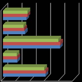
Graph 1 presents scatter diagrams between real GDP and selected right-hand side variables. Real GDP and the real exchange rate exhibit a negative relationship except for the time period when the Argentine government adopted a fixed exchange rate regime. It seems that a relatively high real lending rate tends to hurt real GDP. A higher real oil price tends to correlate with a higher real output. A higher government spending as a percent of nominal GDP tends to associate with a higher real output especially after real GDP reached certain threshold.
According to the DF-GLS unit root test for each of the variables, the critical values are ? 2.5979, ?1.9455 and ?1.6138 at the 1%, 5% and 10% levels.
Comparing with the value of the test statistic, we find that real GDP, the real exchange rate, the real oil price and U.S. real GDP have unit roots whereas the real lending rate, the ratio of government spending to nominal GDP, the real stock price, the current inflation rate, and the lagged inflation rates do not have unit roots. The DF-GLS test on the regression residuals shows that the test statistic of ?2.6148 is greater than the critical value of ?2.6005 in absolute values at the 1% level, Hence, these time series variables are cointegrated and have a long-term stable relationship.
6. Graph 1: Relationships between Real GDP and Selected Variables
Notes: RGDP is real GDP. REXC2 is the real exchange rate. REALLENDR is the real lending rate. ROILPA is the real average oil price. G/NGDP*100 is government spending as a percent of nominal GDP.
Table 1 presents the estimated regression and related statistics. The GARCH model is applied in empirical work. The explanatory power of the regression is relatively high as the value of R-squared is estimated to be 0.8571. The F-statistic of 23.9985 suggests that the whole regression is significant at the 1% level. All the coefficients are significant at the 1% or 2.5% level. Real GDP is negatively affected by the real exchange rate, the real lending rate and the expected inflation rate and is positively affected by the ratio of government spending to GDP, the real stock price, the real oil price and U.S. real GDP. An increase in the real exchange rate indicates that the peso depreciates versus the U.S. dollar. In the short run, a 1% increase in U.S. real GDP is expected to raise the Argentine real GDP by 1.1118%. A 1% real deprecation of the peso versus the U.S. dollar is expected to reduce real GDP by 0.3399%. The wealth effect is confirmed as a 1% increase in the real stock price index would lead to a 0.0548% increase in real GDP through an increase in personal consumption spending and the induced expenditures. The positive significant coefficient of the real oil price suggests that recent declining oil prices have hurt Argentine economic activities. According to the Wald test, the combined coefficients of the current and lagged inflation rates are negative and significant at the 5% level.
To test the impact of fiscal policy, annual data during 1995-2013 for deficit spending and other variables are collected. In Table 2, except for the significant negative coefficient of the expected inflation rate at the 10% level, other coefficients are significant at the 1% level. Regression results show that real GDP has a positive relationship with the ratio of government deficit to GDP, the real stock index, the real oil price, U.S. real GDP and a negative relationship with real depreciation, the real lending rate, and the expected inflation rate. Due to limited number of observations, these results should be interpreted with caution. IV.
7. Summary and Conclusions
This paper has examined the effects of changes in the Argentine peso exchange rate and other relevant business and economic variables on real GDP. Real depreciation of the peso versus the U.S. dollar is expected to reduce real GDP. Furthermore, a higher real interest rate or expected inflation rate hurts real GDP whereas more government spending or deficit as a percent of GDP, a higher real stock price, a higher real oil price or a higher U.S. real GDP would raise real GDP.
There are several policy implications. The Argentine government may need to reassess its exchange rate policy in order to avoid continual peso depreciation as it is harmful to the economy. Argentine authorities may need to consider lowering the interest rate to stimulate consumption spending, investment spending and net exports. As its inflation rate is one of the highest in the world, the monetary authority needs to take measures to reduce inflation expectations in order to stimulate economic activities and protect the wellbeing of the Argentine people. Maintaining a healthy stock market is expected to raise real GDP through the wealth effect.
| Variable | Coefficient | z-Statistic |
| Intercept | 2.4618 | 39.9073 |
| Log(real Peso/USD exchange rate) | -0.3399 | -20.0187 |
| Real lending rate | -0.0009 | -2.4228 |
| Log(government spending/GDP) | 0.3785 | 13.2851 |
| Log(real stock index) | 0.0548 | 5.8000 |
| Log(real oil price) | 0.0368 | 7.2853 |
| Log(U.S. real GDP) | 1.1118 | 217.0860 |
| Current Inflation rate | -0.0036 | -6.6018 |
| Inflation rate (-1) | 0.0024 | 4.9546 |
| Inflation rate (-2) | -0.0024 | -4.4653 |
| Inflation rate (-3) | 0.0001 | 0.1972 |
| R-squared | 0.8571 | |
| F-statistic | 23.9985 | |
| Akaike information criterion | -2.8959 | |
| Sample period | 1996.Q4 -2014.Q2 | |
| Number of observations | 71 | |
| MAPE | 5.6298% | |
| Notes: MAPE is the mean absolute percent error. | ||
| Variable | Coefficient | z-Statistic |
| Intercept | 4.9331 | 20.5989 |
| Log(real peso/USD exchange rate) | -0.3193 | -7.3826 |
| Real lending rate | -0.0025 | -2.6267 |
| Log(government deficit/GDP) | 1.7998 | 5.7071 |
| Log(real stock index) | 0.0758 | 2.9460 |
| Log(real oil price) | 0.1504 | 4.1020 |
| Log(U.S. real GDP) | 0.8762 | 23.4471 |
| Expected inflation rate | -0.0011 | -1.8557 |
| R-squared | 0.9237 | |
| F-statistic | 9.6821 | |
| Akaike information criterion | -2.1930 | |
| Sample period | 1995 -2013 | |
| Number of observations | 19 | |
| MAPE | 4.4602% |