1. Introduction
he new era of information technologies gives me new understanding of retail sales and how they are performing. In nowadays the retail opened a new way of products selling -this is e-commerce. What is ecommerce, how it performs on US market, what new opportunities e-commerce gives to me and how it works? How e-commerce influent on traditional sales, how retail is developing today? These are the topics of my study.
From my understanding the e-commerce sales are a part of retail sales. In other words, e-commerce is simply alternative way of selling and buying products. How new technologies is connected to traditional understanding? From my point of view, I have two parts for investigation. First is -how e-commerce influences on sales via global understanding and trends? Is it produce new opportunities for money moving, is it create new demand? Second, is e-commerce something more modern and advanced, can new technologies replace traditional sales on market?
The first answer is what is e-commerce? Ecommerce, known as electronic commerce, is one of the technological undertakings that have seen companies using computer networks, like the internet, in facilitating trading activities as far as products and services are put into consideration. Electronic commerce brings in such technologies as electronic funds transfer, internet marketing, supply chain management and online transaction processing among others. It should be pointed out that some outstanding transactions that occur under the influence of ecommerce include business-to-consumer, business-tobusiness and consumer to consumer among other operations found relevant.
2. II.
3. Literature Review
Internet marketing and online transaction processing have received significant attention all over the world. According to Monga, the author believes that modern electronic commerce entails the unlimited use of the World Wide Web in the transaction's life-cycle. The author believes that e-commerce can only find ground in businesses through the internet and other relevant network communication technologies. It, therefore, facilitates an automated process of commercial transactions thereby making the operations in business much simpler and easier to handle. Monga looks on the good side of Internet commerce where ecommerce seems to allow people to run their businesses without experiencing any barriers of distance or time. All it demands is to log in the web and access products and services of one's choice.
However, what the author saw to be the most important thing revolved around the impact of Ecommerce on business. It is true that the internet has changed even the way people communicate as well as keep finances. It means that electronic commerce has developed a big impact in the society. Monga fostered on the effects of e-commerce on significant dimensions felt relevant in the business context. She focused on the impact of e-commerce on direct marketing where the author found out that electronic commerce was seen enhancing the promotion of products and services through attractive, direct and interactive contact with clients. It remained paramount that the subject further led to the creation of new sales channel for the popular products and offered a bi-directional nature of communication.
Also, the cost involved in delivering information to potential parties over the net led to substantial savings as far as comparisons between physical delivery and digitized products are in consideration. Monga also focused on reduced cycle time where delivery of digitized products and services could be reduced to a few seconds. Saving time in business is very essential and further defines the performance stand of the business in context. Monga believes that that consumer service can essentially be enhanced given the fact that e-commerce makes it easier for customers to access details online and further forward complaints through email, which can only be done in a few seconds. Apart from easy access to details online, it is also important to look at the corporate image, which is crucial to winning the trust of the clients.
The impact of e-commerce can further be identified regarding manufacturing and finance. The two affect business flow and one should approach these regarding what e-commerce can do to influence their performance in the world of business (Bothma and Geldenhuys). E-commerce is evidently changing most manufacturing systems with pragmatic consideration of the transition from mass production to demand driven as well as just-in-time manufacturing. Most production systems are argued to share integration with marketing, finance, and other systems. Making use of Web-based ERP systems has seen orders taken from customers and directed to designers happening in the shortest time possible. With e-commerce in place, the production cycle time can be cut by almost 50% depending on the type of designers and engineers found in a location.
Jeff Jordan said "we're approaching a sea change in retail where physical retail is displaced by ecommerce in a multitude of categories. The argument at a high level:
Online retail is relentlessly taking share in many specialty retail categories, resulting in total dollars available to physical retailers stagnating or even declining. This is starting to put intense pressure on their top lines.
Physical retailers are very highly leveraged and often have narrow profit margins. Material declines in their top lines make them unprofitable and quickly bankrupt.
Online retail will benefit greatly from the elimination of their physical competition and their growth should accelerate." III.
4. Hypothesis
HOa: E-commerce opens new opportunities to retail sales growth. HOb: E-commerce substitutes traditional sales on market.
5. IV.
6. Data Specifications
The main sources where I found trends are: economic research Federal Reserve Bank site for population, GDP per cap, Households Income, Households dept., Working population, GDP for working population, PPI for US producers and PPI for US Ecommerce; Bureau of Labor Statistics for Employment, Unemployment rate trends; Internet World Statistics site for internet penetration in US; US census site for US retail total sales, stores sales, E-commerce sales, and E-commerce as a Percent of Total Sales.
I tried to obtain all trends in quarter scale for 2000-2015 period. In the end I have problems to find ecommerce within retail category data. That's why data about satisfaction were copied from report.
The Working Population and GDP for working population were found only for 2000Q1-2015Q1 period. I used linear approximation to complete these trends because they have close to linear nature according to graphical examination.
For within retail analysis I found that PPI trend is only for 2006 Q2-2015 Q4 is available. That's why I make time scale for retail analysis shorter. The PPI and PPIE are actually only one measure for retail analysis that was found in quarter scale from beginning from trusted source. I can't drop it, because other scalessatisfaction and penetration for 2000-2015 years have annual scale in reports and were approximated. And sources are not gives me 100% confidence because these scales are taking from survey results, I don't know data and methodology. I understand that these scales Satisfaction and Penetration can be not very good connected because not right scale, and they haven't same regular base of measurement, and only can help me to evaluate general dependence if they present because for such analysis I need real retail data such firm as Nielsen for example, and full consumer's satisfaction research in history. That's why I used these scales approximation for 2006Q2-2015 period only.
V.
7. Conceptual Model
Macroeconomics is a branch of economics dealing with the performance, structure, behavior, and decision-making of an economy as a whole, rather than individual markets. This includes national, regional, and global economies. (Blaug, Mark, 1986;Sullivan, Arthur, Sheffrin, Steven M., 2003).
Macroeconomics deal with such indicators of economy as GDP, unemployment rates, Households income etc. I as macroeconomists can develop models that figure out the relationships between these factors. In my topic I have to include macroeconomic analysis of retail sales by general factors which reflect my understanding of the retail sales, and e-commerce global factors in this model too.
My economic understanding of retail sales value is described as mix of such factors as: size of US market, volume of US market, and the market demands. What I mean when tell this:
The goods are buying by people. This means that population of active consumer's influence on sales volume. How this population can be described? It can be described as total population of US for traditional sales and internet penetration for e-commerce, as base for internet sales.
How I can think about buyers? How buyers influence on sales volume? The buyers go to market and buy goods if they have money to buy and demand. What characteristics of buyers form the volume? The possible answer is GDP, GDP per cap, Income of household, Income of households per cap etc. If I will use general data of GDP or Total income for households I have to adjust this volume using population value, or target population size. Who make sales for retailers? Households?
Or Households + Firms/ Government=GDP? This is interesting question. I propose to check which trend from these two, and select better one.
The other good characteristic of buyers is demand. If people have money but if they needn't to buy goods, they will not buy. If people have demand but they have negative trend (expectations) in economy, the people will try to save money for future. How this parameter can be reflected? If you suffer to lose or find new job you will save money. I propose to figure out this dependence using unemployment rate with lag checking. The total influence of economy is present in GDP/Income data already.
Next good question is about factors of economy which influence on possible volume of sales is situation when I have same economy characteristics in economy but growth of sales. How is this possible? The good example is: if you a man who use e-commerce to sell some needn't goods from home and buy "new". You have same income and GDP approximately (only taxes from e-commerce are added actually), but already have additional not registered income which you can use to buy. The affects like this will describe using US Internet penetration trend. The meaning of such step is that how new technologies rise sales due their development?
Okay, what are the conclusions of upper discussion? I have global factors which influence on retail sales volume. The function for total sales is looking like: Sales = F (Market size (Population), Economy (GDP, income), Demand (Unemployment rate), Ecommerce influence). How this parameter performs. Size multiply on economy value gives the possible volume from which buyers can buy goods. The demand will represent by number of persons which can have demand in goods. The possible trend is unemployment rate, size of target category etc. All that I wrote upper describes my understanding of market to confirm or reject H0a hypothesis, for confirming which I will use US model and trends.
The next understanding describes the process of H0b checking. For confirmation of this hypothesis I will design Retail model and trends. The e-commerce sales are alternative way of buying. This means that within retail, the e-commerce is driven by same understanding in general but I will use other trends which reflect this understanding within retail. The main definitions are: Market size, market values -economy, demand -the benefits of e-commerce use, other unexplored influences. Which data/trends were selected to determine this influence in my study?
The size factor is coverage: internet penetration, count of e-shop's buyers etc. Can I buy product if I'm not internet user and don't know how to make this? Of course not! During my mining process I found only one trend -internet penetration. The number of shops, its volume, and count of e-shop's buyers are information which can be bought only as part of retail researches provided by marketing agencies.
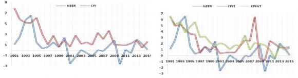
The most powerful driver on market in all times is when your products in your shops are affordable/cheaper than others. To investigate this factor, I have to find trend which reflects economy. According to economic theory this can be price elasticity or differences in prices. If proposition in your e-shop is better than in traditional the people will like to buy goods in your shop. If goods produced by your industry is cheaper than they are more concurrent. During my investigation I found only Producers price index (PPI) as part of governmental statistics. The Consumers price index (CPI) was found only for total retail. The CPI for ecommerce goods can be obtained only in marketing agencies again.
Demand? Why I have to buy goods in Ecommerce shops? Why I need to do this? The possible answer is a satisfaction about e-shops use compare to other solutions. This trend has to include emotional, functional and other benefits characteristics of e-shops usage. This topic is a part of special researches again. But I found report which have satisfaction trend in annual scale to reflect my understanding.
8. VI.
9. Data Analysis
The data analysis includes the trends analysis which I found according to description from conceptual model. How these data were transformed and computed to reflect my economic understanding. According to model I have two steps, two regression models. First is reflecting the US market understanding/prediction of US retail sales to find the influence of e-commerce on global level. Second is working within US retail to figure out how e-commerce is performing as alternative way of buying. In other words, my model can be used for prediction, forecasting, or to study the relationships between the independent variables and the dependent variable, and to explore the forms of these relationships (Armstrong, J. Scott, 2012).
According to upper discussion I found such trends: Total retail sales, Stores sales, E-commerce sales, E-commerce as a Percent of Total Sales in quarter scale for 2000-2015 years. These trends are representing retail data for both parts of analysis. According to understanding of regression analysis I have to make 5 steps of data analysis: Data validation, Data transformation, Correlation analysis, Outliers identifying, Checking multivariate assumptionsnormality.
10. VII.
11. Data Validation
This is the process which validate can be trends used in model to logical criteria.
The employment trend can't be used because it is reflected in percentage of population. This measure is not reflecting the aging. This means that this parameter is dropping people in high age as not consumers. But this is not connected to real situation. Thus only unemployment rate can be used.
CPI is not used because I have not found same statistics for e-commerce. Households dept. was dropped because household's income trend shows lower correlation in future correlation analysis.
Working population is dropped because it not reflects total consumer population means target category of analysis.
I found other trends except listed in data analysis part. But they are not passed validation process.
I continued with the overview of and checked for potential multicollinearity issue, skewness and kurtosis issue. From the rule of the thumb I can estimate that I'm having challenge with skewness and kurtosis. I run a description analysis for this:
12. B
The Impact of E-Commerce on Retail Harrell discusses a lot of options for "dimension reduction" (getting your number of covariates down to a more reasonable size), such as PCA, but the most important thing is that in order to have any confidence in the results dimension reduction must be done without looking at the response variable. Doing the regression again with just the significant variables, as you suggest above, is in almost every case a bad idea". (Harrell, Frank., 2001).
In my analysis I have 64 observations for US trends. That's why I can use 3 or 2 trend model for linear regression.
For second part which describes retail trends I have to use 2 trends for good estimation and VIII.
13. Data Transformation
The example I have US GDP per capita and population. This data has to be multiplied according to understanding of market volume = size * value.
The penetration value has to be transformed into volume value same as in previous paragraph.
The unemployment rate is in percentage. And it has not to be transformed because according to my plan it has to reflect the demand -value between 0 and 1 when 1 there is not demand present when 0 people buy all that they can. Of course other trend of demand may be found through market researches according to customers spent survey or something like this. But current trend looks good in my logic too.
I predict a percent of e-commerce sales to find, how this factors substitute traditional retail. The data difference in satisfaction and difference in PPI are not implemented directly. It demonstrates a moving process of shoppers according to perceptions. The moving process is connected to importance of e-commerce for people and advertising. The best trend which reflects the importance of e-commerce sales within retail is ecommerce sales value. So I decided to multiply ecommerce sales from previous period on this difference to reflect this understanding correctly. In other words, people who are using e-commerce can describe to others why they are using it, and agitate them to use this way of buying.
The other problem is difference in data measurement scale. When I multiply GDP per capita on Population I received a big number. I decided to divide it on 10-4 to make regression coefficients more comfortable to view and understand.
14. IX.
15. Correlation Analysis
I have to check are my variable related to each other somehow? To make this, I used Pearson correlation. The most familiar measure of dependence between two quantities is the Pearson product-moment correlation coefficient, or "Pearson's correlation coefficient", commonly called simply "the correlation coefficient". It is obtained by dividing the covariance of the two variables by the product of their standard deviations. Karl Pearson developed the coefficient from a similar but slightly different idea by Francis Galton. (Rodgers, J. L.; Nicewander, W. A., 1988).
I carried on with the correlation examination in order to find out the relationships between predicting variables to select better one list of trends.
I analyzed bigger number of trends when searching for appropriate data and model. But last trends are reflecting model well, I used few from others to demonstrate selection process. According to table 3 I have 10 trends related to our data. I have to select only needed. For example, I have trends which described Income. This is GDP per capita, GDP work -GDP for working part of society. According to this tables GDP per capita have highest correlation, thus I decide to select it as trend for analysis. Next I see that population trend have big correlation value too. But in my understanding my model in logic purposes can't be like a*pop + b*gdp per cap because these data have to be connected via multiplying to show the total volume. That's why GDPpop4 trend was designed. The unemployment rate was selected instead Employment because I select total population instead working population and only this trend relate to these data. The penetration represents the measure of high technology understanding in society, to outline how connection to internet and its usage lead people to use new capabilities. This parameter helps to understand how understanding (4) performing in US model.
16. XI. Checking Multivariate Assumptions -Normality
According to understanding of model I are not searching for one value, which is true. I want to examine all diapason. That's why my trends have to be not normally distributed, or better say maximum scattered.
17. B
The Impact of E-Commerce on Retail
18. Regression Models
In statistics, linear regression is an approach for modeling the relationship between a scalar dependent variable y and one or more explanatory variables (or independent variables) denoted X. The case of one explanatory variable is called simple linear regression. For more than one explanatory variable, the process is called multiple linear regression (David A. Freedman, 2009).
19. XIII.
20. Why i used Multiple Linear
Regression?
In my model I am sure that data have linear relations with dependent variable, because this leads from my conceptual model which was built on real economic understanding and logic of market, and trends transformations which were made to represent data in same scale and same logical understanding according to conceptual model for US's and Retail's regression models.
21. XIV.
22. US Regression Model Results
23. Table 7 : US Model Summary
In Table 7 of US Model Summary I see that R Square = 0.954. I could explain 95.4% of variability in the dependent variable with this multiple linear regression model according to the model summary. This is what exactly I needed, because I want to receive model which is close to real life.
According to ANOVA table 8 in this multiple linear regression model is a statistically signi ficant predictor of the dependent variable, with p-value = 0,000 (which significantly below the 0.05 critical value). According to Table 9, I have 2 statistically significant coefficients. This is GDPpop4 and Unemployment Rate. The Penetration is not statistically significant. This means that penetration has not statisticaly significant influence on this model (or very small which can't be recognized), and can be excluded if I want to build equation for model.
Backing to my hypothesis I have to reject HOa that E-commerce opens the new opportunities to retail sales growth, or they are not significant. In other words, internet usage and internet penetration not leads to changes and raising retail sales significantly.
There is variance inflation factor VIF that explains colinearity level between independent variables that is quite higher than 10 meaning there is not colinearity level between independent variables for GDPpop4 and penetration. This is bad result.
I re-run US model and I excluded penetration variable to obtain better equation for Retail sales. There is variance inflation factor VIF that explains collinearity level between independent variables that is quite lower than 10 meaning there is collinearity level between independent variables for GDPpop4 and penetration.
All other possible outputs are great too. This means that I can use this second US model without influence of Internet penetration to predict sales volume. Backing to my hypothesis I have to accept HOb: E-commerce substitute traditional sales on market. What drivers of this process and how are they measuring? I find that positive differences in satisfaction and Producers index leads to popularizing of shopping.
24. XV. Retail Regression Model Results
There is variance inflation factor VIF that explains collinearity level between independent variables that is quite lower than 10 meaning there is collinearity level between independent variables for SalesGrapPPIDif2 and CurSatDif. This is good.
25. Plot 1 : Normal P-P Plot of Regression Standardized Residual
The Plot 1 shows the differences between observed and estimated value. I see there that I have some disconnection from my point of view. I will describe this in conclusions better.
I also checked for homoscedasticity issues of my database as show and according to the graphical examination from where I can conclude that I haven't got problem with heteroscedasticity (Goldberger, Arthur S., 1964).
26. B
The Impact of E-Commerce on Retail
27. XVI. Conclusion and Recommendation
As results, I have to reject HOa: E-commerce opens the new opportunities to retail sales growth, and how is this measuring? This measurement, according to results, is not significant. Possible I can find some other trends but internet access and growing number of internet users are not gives significant impact on retail volume.
The retails sales are measuring according to general understanding of economics. According to demand. The possible formula to obtain significant value of US retail is:
Population*10-3 *GDP per capita *2.581695207*10-4 + Unemployment Rate %*-8609.253793 -102862.6385 = sales. The minus value of constant can be explained as minimum level of market volume needed + expectations to start retail sales. According to this analysis I can recommend to develop e-commerce solutions like in paragraph (4) of conceptual model to obtain influence which will significant. But for now such influence on market are not significant.
According to results I have to accept HOb: Ecommerce substitute traditional sales on market. What drivers of this process and how are they measuring? The drivers of this process is higher satisfactions of using e-commerce and differences in prices. The PPI of e-commerce firms is lower. That's means that goods and services are cheaper and affordable compare to traditional solution. The other conclusion is that if you use internet, this does not mean that you use ecommerce. But you begin to use ecommerce if somebody who use it already recommend and describe you the profits in price and satisfaction.
The formula for e-commerce percentage in retail sales is: (SatisfactionE-commerce%-SatisfactionTraditional%)*E Sales*7.731388+(PPI-PPIE ) *ESales* 0.652988531 +0.003371% = ESales%.
This formula tells me that Positive satisfaction and positive difference in sales index between Ecommerce and Traditional attributes leads to growth of ESales. If difference become "-", then I will have observed decreasing of E-commerce percentage. I find that E-commerce sales is driven by consumer's logic, and not connected to popularization of information technologies, only to economic logic.
28. XVII.
29. Further Research
The further investigations can deal only with more concrete data which can be obtained only in marketing agencies which conduct retail researches.

| How many observations I have to have in my |
| models. The scientific criteria are: "The general rule of |
| thumb (based on stuff in Frank Harrell's book, |
| Regression Modeling Strategies) is that if you expect to |
| be able to detect reasonable-size effects with |
| reasonable power, you need 10-20 observations per |
| parameter (covariate) estimated. |
| N | Minimum | Maximum | Mean | Std. Deviation | Variance | Skewness | Kurtosis | |||||||||
| Statistic | Statistic | Statistic | Statistic | Std. Error | Statistic | Statistic | Statistic | Std. Error | Statistic | Std. Error | ||||||
| Working Population | 64 | 178274.000 | 207535.595 | 194140.345 | 1005.496 | 8043.970 | 64705455.964 | -.418 | .299 | -.929 | .590 | |||||
| Unemployment Rate | 64 | 3.800 | 10.000 | 6.295 | .223 | 1.788 | 3.195 | .688 | .299 | -.775 | .590 | |||||
| Population | 64 | 281304.000 | 322693.000 | 302622.234 | 1535.440 | 12283.520 | 150884875.230 | -.079 | .299 | -1.234 | .590 | |||||
| Employement | 64 | 58.200 | 64.700 | 61.150 | .271 | 2.172 | 4.717 | -.114 | .299 | -1.635 | .590 | |||||
| GDPPC | 64 | 12359.100 | 16470.600 | 14451.189 | 140.710 | 1125.679 | 1267153.134 | -.233 | .299 | -.861 | .590 | |||||
| GDP Work | 64 | 2203306193.400 | 3349511675.586 | 2811181894.911 | 40606814.525 | 324854516.202 | 105530456696851000.000 | -.295 | .299 | -.953 | .590 | |||||
| GDP pop | 64 | 3476664266.400 | 5314947325.800 | 4386380689.352 | 63988993.812 | 511911950.494 | 262053845058295000.000 | -.108 | .299 | -.947 | .590 | |||||
| GDPpop4 | 64 | 347666.427 | 531494.733 | 438638.069 | 6398.899 | 51191.195 | 2620538450.583 | -.108 | .299 | -.947 | .590 | |||||
| Penetration | 64 | 43.100 | 88.910 | 69.326 | 1.524 | 12.194 | 148.682 | -.481 | .299 | -.168 | .590 | |||||
| Sales | 64 | 715102.000 | 1187169.000 | 975369.219 | 16185.214 | 129481.712 | 16765513697.412 | -.127 | .299 | -.774 | .590 | |||||
| Valid N (listwise) | 64 | |||||||||||||||
| Std. | ||||||||||||||||
| N | Minimum | Maximum | Mean | Deviation | Variance | Skewness | Kurtosis | |||||||||
| Std. | Std. | Std. | ||||||||||||||
| Statistic | Statistic | Statistic | Statistic | Error | Statistic | Statistic | Statistic | Error | Statistic | Error | ||||||
| SalesGrapPPIDif2 | 39.000 | 0.017 | 0.064 | 0.039 | 0.003 | 0.016 | 0.000 | 0.108 | 0.378 | -1.563 | 0.741 | |||||
| CurSatDif | 39.000 | 0.002 | 0.003 | 0.002 | 0.000 | 0.001 | 0.000 | 0.659 | 0.378 | -0.906 | 0.741 | |||||
| Penetration | 39.000 | 68.675 | 88.910 | 76.888 | 1.084 | 6.767 | 45.794 | 0.625 | 0.378 | -1.235 | 0.741 | |||||
| PercentOfESales | 39.000 | 0.027 | 0.075 | 0.047 | 0.002 | 0.014 | 2.007 | 0.498 | 0.378 | -0.954 | 0.741 | |||||
| Valid N (listwise) | 39.000 | |||||||||||||||
| SalesGrapPPIDif2 | CurSatDif | Penetration | PercentOfESales | |||
| SalesGrapPPIDif2 | Pearson Correlation | 1 | .775 ** | .867 ** | .952 ** | |
| Sig. (2-tailed) | .000 | .000 | .000 | |||
| N | 39 | 39 | 39 | 39 | ||
| CurSatDif | Pearson Correlation | .775 ** | 1 | .945 ** | .848 ** | |
| Sig. (2-tailed) | .000 | .000 | .000 | |||
| N | 39 | 39 | 39 | 39 | ||
| Penetration | Pearson Correlation | .867 ** | .945 ** | 1 | .908 ** | |
| Sig. (2-tailed) | .000 | .000 | .000 | |||
| N | 39 | 39 | 39 | 39 | ||
| PercentOfESales | Pearson Correlation | .952 ** | .848 ** | .908 ** | 1 | |
| Sig. (2-tailed) | .000 | .000 | .000 | |||
| N | 39 | 39 | 39 | 39 | ||
| **. Correlation is significant at the 0.01 level (2 -tailed). | ||||||
| X. | Outliers Identifying | |||||
| I continued with graphical examination in order | ||||||
| to visually detect missing data, outliers in influential | ||||||
| points. | ||||||
| 2016 |
| Year |
| Volume XVI Issue V Version I |
| Global Journal of Management and Business Research ( ) B |
| XII. |
| Kolmogorov-Smirnov a | Shapiro-Wilk | |||||
| Statistic | df | Sig. | Statistic | df | Sig. | |
| SalesGrapPPIDif2 | .145 | 39 | .038 | .902 | 39 | .003 |
| CurSatDif | .153 | 39 | .023 | .883 | 39 | .001 |
| Penetration | .225 | 39 | .000 | .851 | 39 | .000 |
| PercentOfESales | .124 | 39 | .136 | .929 | 39 | .017 |
| a. Lilliefors Significance Correction | ||||||
| According to ANOVA table 12 in this multiple |
| linear regression model is a statistically significant |
| predictor of the dependent variable, with p-value = |
| 0,000 (which significantly below the 0.05 critical value). |
| Standardized | Collinearity | ||||||||||
| Unstandardized Coefficients | Coefficients | Correlations | Statistics | ||||||||
| Zero- | |||||||||||
| Model | B | Std. Error | Beta | t | Sig. | order Partial Part Tolerance | VIF | ||||
| 1 | (Constant) | -714922.523 | 222746.132 | -3.210 | .002 | ||||||
| Employement | 8070.848 | 2897.795 | .135 | 2.785 | .007 | -.728 | .336 | .081 | .360 | 2.780 | |
| GDPpop4 | 2.728 | .123 | 1.079 | 22.191 | .000 | .970 | .943 | .647 | .360 | 2.780 | |
| a. Dependent Variable: Sales | |||||||||||
| Minimum | Maximum | Mean | Std. Deviation | N | |
| Predicted Value | 3.0339% | 6.8710% | 4.7077% | 1.37117% | 39 |
| Residual | -.45409% | .76846% | .00000% | .35627% | 39 |
| Std. Predicted Value | -1.221 | 1.578 | .000 | 1.000 | 39 |
| Std. Residual | -1.241 | 2.099 | .000 | .973 | 39 |
| a. Dependent Variable: PercentOfESales | |||||