1. Introduction
o classify every entity as perishable or not, we need to establish the threshold value for the shelf life. Examination of the data has revealed that all products which require a conditioned environment have a shelf life that is equal to or less than 30 days (Donselaar et. al., 2003). Consequently, in this paper we have defined perishable life of the product as less than or equal to 30 days. K. van Donselaar (2003) applied this definition to the entire assortment (including here weight products and direct deliveries) in his paper and estimated that roughly 15% of the assortments are perishables versus 85% non-perishables. Commodities that have predetermined useful life are said to be perishable commodities (Gupta et. al., 2003). Common examples include decomposing organic products such as vegetables, fruits, daily bread, milk and meat etc. Perishable commodities may also have fixed life time, after which they are not useful for the use, such as medicines, packaged juices (for which lifetime is different when opened) etc.
Our paper is based on already published two papers in which discounts are offered and they have (Sezen, B., 2004, Ramanathan, R., 2006). In our paper we have considered only "egg" as a perishable product since it is a commodity which is used as a regular item in the household and have a seasonal lifetime of 2-5 weeks which is close enough to analyze the discount approach of Sezen (2004) and Ramanathan (2006).
2. II.
3. Literature Review
Numerous models have been developed in literature so that inventory management of perishable products can be easily understood and it can be useful in accepting complex situations of perishability. Some complex models including returns policies (Vlachos, D. and Dekker, R. 2003, Hahn, K.H, et. al, 2004), ordering policies for cyclic commodities (Gupta et. al., 2003), demand with time variance, production and deterioration rates (Goyal, S.K. and Giri, B.C., 2003) have also been developed in the literature.
Problem related to discounting and stocking decisions for short shelf life perishable commodities has not attained the due magnitude in literature (Ramanathan, R., 2006). Decisions regarding discounts have been considered in some somewhat old articles, while there seems to be an improved interest in taking into account discounting policies in some recent articles (Arcelus, F.J., 2003, Sezen, B., 2004, Ramanathan, R., 2006). Abad (2001), with an objective of profit per period, allows for elastic pricing, assuming that the perishables are price sensitive. His procedure is relatively simple and can be implemented on a spread sheet. Similarly, in a different inventory model of Abad (2003), the decision variable is the selling price of the product. Teng et al. (2007) have widened his model with additional costs of backlogging and lost goodwill. Tsao and Sheen (2008), with the same intention of maximizing net profit; show that dynamic decision-making is superior to fixed decision-making in terms of retail price and promotional effort. In practice, it is common to put forward deteriorated items at a discounted price. In many supermarkets, items that are near their expiration date are marked down by a fixed percentage to Monitoring and organizing of perishable products can be facilitated by the applying radio frequency identification (RFID) and a policy of dynamic pricing (Berk, E. et. al. 2009, Bisi, A. andDada, M. 2007), such as discounts when the item reaches a predetermined age. Ferguson and Koenigsberg (2009) discuss the probable cannibalization effect of having both highpriced fresh products and low-priced older products in same shelf. Ramanathan (2006) and Sezen (2004) assume two discount rates for the first and second discount period in their models. Arcelus et al. (2003) provide a model with payment reduction schemes other than temporary price discounts. They presume that the vendor's trade advertising is a mix of credit and/or price discount. For the retailer, the model determines the size of the special order to be placed at the vendor, the price and/or creditterms incentives to be passed onto customers and the quantity to be sold under these one-time-only situations. In the model by Tsao and Sheen (2007) the price discount is a function of both quantity and time of order placement whereas Lin et al. (2009) presume a selling price that decreases linearly with time and customer demand linearly increases with the same. Sezen (2004) provides an interesting procedure to empirically identify optimal discounting policies for perishable commodities and is further elaborated by Ramanathan (2006). Sezen (2004) has used expected profit approach to identify the timing and quantum of discount for perishable commodities while Ramanathan (2006) used probability distributions to justify the probability of selling the perishable product along with no. of units to be stocked. Ramanathan (2006) extends the expected profit approach from Sezen (2004) by including decisions on the quantities of the perishable products to be stocked by the retailer.
This paper attempts to extend the expected profit approach presented in Sezen (2004) & Ramanathan (2006) by including decisions on the quantities of the perishable products to be stocked by the retailer and adding the cost incurred variable holding cost, cost of revenue/waste generated after the end of shelf life. Their findings are duplicated with data taken from wholesalers who sells perishable commodity like eggs.
Section 3 deals with the objectives and methodology followed by us in this paper. Section 4 will propose the expected profit equation with notations followed by Sezen (2004) and Ramakrishnan (2006). Section 5 deals with data collected from the wholesale market and use of Monte-Carlo simulation technique to analyze the best possible discount period, with specifically eggs taken as perishable commodity with summarized results. Section 6, is conclusions and future research directions.
4. III.
5. Objectives and Methodology
As discussed earlier, this study is the continuation of two previous studies (Sezen, B., 2004, Ramanathan, R., 2006) in which they have considered a perishable commodity of shelf life 30 days. In our study we are extending this by taking revenue/waste cost after the shelf life of the product has expired. We are also considering variable holding cost as this was not the case for the studies done earlier. Keeping this in light, our objectives are: ? To optimize the number of items to be stocked by the wholesaler seasonally and the quantum of discount to be offered.
? To identify the best possible time to offer the discount.
? To minimize the unsold inventory and hence maximize the profit.
As we know that the demand patterns for such type of commodities cannot be exactly known. Stochastic demand patterns are considered as closest way to analyze the situation in terms of perishable products. Such demand patterns are considered very rarely in the literature (Gurler, U. and Yuksel Ozkaya, B. 2003, Berk, E. et. al. 2009, Li, Y. et. al. 2011). After discussing with the wholesalers, we understand that approximately 65-70% of their demands are constant throughout year due to fixed retailer market. Therefore we have taken 70% demand pattern for normal period of sales to make our calculations easier. Demand for first discounted period as well as for units unsold even after discount are randomly generated using the RAND command in excel. Since we have considered probability distribution as arbitrary, again RAND command in excel is used to generate the probabilities for the respective periods of normal demand, discounted demand, and unsold demand.
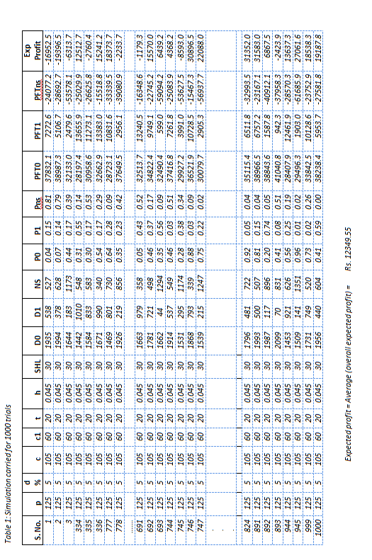
The excel sheet for monte-carlo simulation is run for 1000 trials for profit, making the demand and probability pattern selection totally random. In using a Monte-Carlo modeling approach, a higher number of realizations usually leads to a more reliable and convergent result. Results are said to be converged if the estimate of a particular percentile value does not change significantly if additional Monte-Carlo simulations are performed. However, it is not generally possible to determine beforehand how many realizations are needed to achieve a specified degree of convergence since the value can be highly dependent Year ( )
1 2014on parameter distributions. Once profit and the probabilities of all the combinations of D0, D1 are (table 1). computed, the expected profit can be calculated If the demand patterns during normal and discount period are assumed to be independent, then the probability of obtaining the above decisions for perishable commodities over profit is the product of P(D0), P(D1) and P(NS) (Ramanathan, R., 2006). Once profit and the probabilities of all the combinations of D0, D1 and DNS are computed, the expected profit can be calculated. This expected profit provides a guide for the choice of the number of units to be stocked (n), appropriate times (t) of beginning the discount and the quanta of discounts (d).
IV. Proposed Expected Profit Approach for Stocking and Discounting Decisions
We consider one discount period in this model. In view of the fact that it is not possible for the wholesaler to give extra discount due to short shelf life of the product. To provide continuity, we have attempted to use, as far as possible, the same notations used by Sezen profit per unit when the product is sold in the normal (no-discount) period PFT1 -profit per unit when the product is sold during the discount period PFTns -loss per unit when the product is not sold in any period but can have resale resulting in some revenue.
Items are placed on shelf for sale at time 0 and sold at price P without any discount during the normal period (time 0 to time t). If there are items unsold at the end of a pre-specified period t and until the shelf-life of the product, discount policy is applied to encourage consumers buy before the product expires. If the product is sold between the time period t to SHL, a discount d is applied so that the selling price is p x (1d). In our paper, we have assumed the following: ? All arriving items are new and their lifetime starts when they are placed on the shelf;
? The unsold products at the end of shelf-life are disposed with some extra cost or revenue.
6. ? Purchase cost c is constant.
? There is a fixed demand rate in normal period for both summer and winter seasons.
7. a) Mathematical Relationships
During the total shelf life of the product, we assume three time phases in which three different prices can be applied. The first period, the normal (nodiscount) period, is the time between the placement of the egg crates on the shelf and the start of the first discount at time t. The selling price in the normal period is p. The second period, the discount period, is the time in which the discount price is applied until the end shelf life of the eggs. The selling price in the first discount period is equal to p (1-d), where d is the discount rate for this period. Finally, the last period, where the product is not sold even after offering discount, occurs after the end of shelf life.
In a local market such as Aligarh, cost of waste is negligible due to the fact that expired; unsold eggs are thrown away in bins. Hence we have taken the cost of waste as negligible as it does not affect the overall cost of the wholesaler. The profit for normal period can be calculated as: PFT 0 = {(selling price) -(purchasing cost + average holding cost)} x no. of units sold in normal period
= {p -(c + t x h / 2)} x D 0Here, since we do not know the precise moment in time of selling the product, the average holding cost is roughly found by taking the half of t and multiplying the result by the unit holding cost h. For the first discount period, the selling price is discounted by the rate d. In addition, if the product is sold in the discount period, the holding cost will rise because the product is carried beyond the normal period. Therefore, profit per unit for a product sold in the first discount period is calculated as follows:
PFT 1 = p 1 -d -(c + t x h + ((SHL ? t)x h) ÷ 2) x D1Since the product is held (not sold) until the first discount period, inventory holding cost is the sum of inventory costs for the entire normal period (t x h) and the half of the unsold period.
In case where the manufacturer is able to return the unsold item back to other manufacturer then it can be accounted for revenue. It simply reduces the cost of the wholesaler. Some local bakery manufacturers often buy from them in order to serve their needs and reduce the overall costs of buying. Sometimes, big wholesalers put pressure on "mandis" i.e. local poultry markets, to take the lot of waste eggs back and charge a small amount for their disposal for next lot. These eggs are sold to the manufacturers of poultry feed at a lower cost. Therefore, we have tried to inculcate such cost also. This additional cost can be termed as revenue for the wholesaler's. It can be denoted as:
8. R= NS x c 1
where c 1 <c When the product is not sold in any of these periods, in that case, instead of a profit value we find a quantity of loss and may generate some revenue. The equation will be:
9. PFTns = Revenue -(cost of the lot unsold + holding cost) = {c1 -(c + (SHL)x h)} x NS
Here, ShL x h gives us the total holding cost for the product because it is kept on the shelf until the end of its expiry date. We assume that the cost of removing and disposing the unsold products is negligible.
For any given discount rate and time combination (d, t), assume that P 0 , P 1 are the probabilities for selling a product in the normal period, discount period respectively. Further, assume that Pns is the probability of not selling the product. Since these probabilities (P 0 , P 1 and Pns) are collectively exhaustive, that is, at least one must occur in any condition, their total should be 1. With these probabilities and the profit per unit values, the expected profit can be found by using the common expected value approach (Ramanathan, R., 2006):
(Expected profit) i = P 0 (PFT 0 ) + P 1 (PFT 1 ) + Pns(PFTns)
Therefore for 1000 trials expected profit is the average of all the scenarios randomly generated, which can be represented as:
Average Expected profit = ? ( ) V.10. Data Analysis
In India, egg is a commodity used in large quantity which has a short shelf life. As Sezen ((Sezen, B., 2004)) & Ramanathan ((Ramanathan, R., 2006)) tried to support their mathematical relations through assumption of data, we have tried to take the required inputs through wholesaler markets here in Aligarh, India. Egg has a lifetime depending upon the season cycle; hence two type of analysis has been carried out so that both seasonal discounts can be taken into consideration. For summer season shelf life of eggs are approximately 15 days whereas in winter season 30 days shelf life is considered. Example here is carried out for winter season, when the shelf life of an egg is approximately 30 days. Data taken under consideration is an average for four wholesalers. They procure eggs from different markets known as 'Mandis', which in turn buy from poultry farms all across Aligarh and nearby areas.
Example: For winter season-shelf life 30 days.
In our case, as we have considered only one discount period, no of days are limited to t -(20, 25 days) with discount values d -(5%, 10%, 15%, 20%). No of items to be stocked are substituted as n -(2000, 3000, 4000, 5000 crates per lot). Holding cost per unit is also calculated as illustrated below. Demand for 1 st period, i.e. normal period is assumed to be approximately 70% of overall demand; following calculations are done (Table 1) with data as under. Table 1 shows the overall 1000 trails carried in excel for generation of the average expected profit. The expected profit for the 1 st scenario (as shown in table 2) can be calculated as:
PFT 0 = {125 -(105 + 20 x 0.045 / 2)} x 1935 = Rs. 37832.1Similarly PFT1 and PFTns is calculated and expected profit is
(Expected Profit) i=1 = P0x(PFT0) + P1x(PFT1) +Pnsx (PFTns) = 0.04x37832.1 + 0.15x7272.6 + 0.82x(-24077) = -16952.5Therefore for 1000 trails, average of Expected profit is:
Average Expected Profit = ( ???.. ) = Rs. 12349.55The overall summarized table for different discount rates, time of discounts and the no of units to be ordered are shown in table 1.
11. Global Journal of Management and Business Research
Volume XIV Issue III Version I Year ( ) A For summer season (table 2), major problem for the wholesaler is the limited shelf life of eggs. Also the demands are less. Therefore it is better to stock at a level where losses can be reduced and chances for losses are minimized. One such scenario can be seen in For n=1000, d=15% and t= 8 th day, we can see that the wholesaler's average profit is maximum Rs. 3807.2 with a positive profit chance of 84.8%. Also the losses are not high in this case. Another close scenarios are when (n,d,t); (3000, 0, 0) and (4000, 5%, 10). In both these cases, first inventory is quite high, which involves stocking, distribution cost along with additional sale requirement. Also, positive profit chances for both the cases are 67.8% and 68.0% respectively. Also the loss incurred is huge. Therefore, in summer season, where the wholesaler do not have large shelf life, the best possible combination for number of units to be stocked, quantum of discount and time of discount will be n=1000, d=15% and t=8 th day.
For winter season (table 3), due to the enhanced shelf life of the egg, it is easier for the wholesaler to stock more and more. Since at n=3000, d=5% and t=20 days, we see that average profit comes out to be Rs. 13349.50. The chances of maximum profit will be Rs. 39883.3 and maximum loss will be Rs. 48167.40. Close to the highlighted figure (table 3), are (n,d,t); (3000, 5%, 25) , (4000, 5%, 20), (5000, 5%, 20) and (5000, 5%, 25). But, as we can see, the minimum value of profit are quite high and chances of profit are also low when compared to (3000, 5%, 20). Same is the case with inventory for 4000 units and 5000 units. Additionally such large inventory will require more marketing, sales, distribution, storage etc. which will inculcate extra cost and pressure on the wholesaler. Table 2 : summarized results for summer season Therefore, in winter season, where the wholesaler has the liberty of having shelf life of 30 days, the best possible combination for number of units to be stocked, quantum of discount and time of discount will be n=3000, d=5% and t=20 days. Another interesting fact is, the average profit at n=5000, d=0% and t=0% is Rs. 15643.6, see that the difference of maximum and minimum values of profit is quite large. Also the probable chances of having profits are 68% approx which is quite less as compared to the optimum scenario. Hence it is not a wise decision for wholesaler to carry on with large amount of eggs with lower discounts. The simple expected profit calculation procedure depicted in this study could be utilized at least for two reasons. The first reason might be to compare a discount policy with a no-discount policy. In table 2 and table 3, for example, we can easily make a decision in favor of applying a discount policy instead of a no-discount policy. Another reason could be to evaluate several different discount rate combinations and/or various discount schedules for a number of crates need to be ordered. As we can see from the result table that offering discount is somehow better than not offering discounts in both seasons. Although in some cases no large difference in revenue is there between zero and some discount offered by the wholesaler, but the chances of profit/ loss also effects the decision. On the other hand, when they are implemented in the right manner, price discounts offered for eggs in both seasons have their own benefits like reduction of waste; shortening the cycle time for the item inventories and thus, more space availability for the fresh products; and reduction of the holding costs. Hence, there appears to be a tradeoff between the benefits of perishable product discount pricing and the costs linked with the challenging full-priced perishable products. Achieving a well-balanced pricing approach will require information regarding the characteristics of the specific market, including the percentage of waste of perishable products, the proportion of discounted perishable products, and the customers who wait for the discounts (which are price sensitive). Only with such information, the true impact of perishable item discount pricing on the demands of other products could be determined.
For future research, more trials can be performed in order to reduce the chances of errors. Cost of waste can also be inculcated in the equation. Other factors such has producer's risk and consumer's risk can also have an effect on the overall performance of wholesaler. Also other factors effecting demand such as economic, demographic etc. can be taken care of for future research.

| SHL-15 days | |||||||
| N | d | t | Average | Max | Min | Positive | Negative |
| 1000 | 5% | 8 | 3477.3 | 8965.6 | -9256.3 | 83.6% | 16.4% |
| 10 | 3281.1 | 8926.8 | -9487.3 | 83.5% | 16.5% | ||
| 10% | 8 | 3694.8 | 8973.3 | -7367.3 | 84.5% | 15.5% | |
| 10 | 3261.0 | 8939.6 | -9104.1 | 84.5% | 15.5% | ||
| 15% | 8 | 3807.2 | 8965.5 | -7411.1 | 84.8% | 15.2% | |
| 10 | 3677.2 | 8939.8 | -9001.1 | 78.5% | 21.5% | ||
| 0% | 3614.1 | 9096.8 | -8011.2 | 80.7% | 19.3% | ||
| 2000 | 5% | 8 | 3515.5 | 17219.9 | -31465.4 | 74.2% | 25.8% |
| 10 | 3716.7 | 17626.5 | -31468.1 | 72.5% | 27.5% | ||
| 10% | 8 | 3370.4 | 17178.3 | -29925.6 | 71.2% | 28.8% | |
| 10 | 3159.0 | 17300.5 | -36712.2 | 72.7% | 27.3% | ||
| 15% | 8 | 2979.4 | 17794.6 | -30609.8 | 66.3% | 33.7% | |
| 10 | 2979.4 | 17216.2 | -30505.5 | 67.1% | 32.9% | ||
| 0% | 3303.6 | 17681.1 | -37309.1 | 64.8% | 35.2% | ||
| 3000 | 5% | 8 | 3557.4 | 25445.5 | -69030.3 | 70.3% | 29.7% |
| 10 | 2618.3 | 25820.3 | -61678.9 | 68.2% | 31.8% | ||
| 10% | 8 | 2658.2 | 25459.0 | -51131.2 | 66.2% | 33.8% | |
| 10 | 2922.2 | 26237.4 | -61770.0 | 65.5% | 34.5% | ||
| 15% | 8 | 1753.3 | 25868.8 | -52024.0 | 63.5% | 36.5% | |
| 10 | 1753.3 | 26304.8 | -55396.9 | 66.6% | 33.4% | ||
| 0% | 4963.2 | 27172.1 | -55772.9 | 67.8% | 32.2% | ||
| 4000 | 5% | 8 | 3995.3 | 35289.4 | -74373.2 | 66.8% | 33.2% |
| 10 | 4728.9 | 35087.7 | -88833.2 | 68.0% | 32.0% | ||
| 10% | 8 | 2515.7 | 34680.8 | -79402.2 | 64.4% | 35.6% | |
| 10 | 2781.0 | 34142.0 | -76772.3 | 64.6% | 35.4% | ||
| 15% | 8 | 957.7 | 34116.8 | -83055.6 | 61.9% | 38.1% | |
| 10 | 957.7 | 34141.5 | -82286.9 | 61.9% | 38.1% | ||
| 0% | 4327.3 | 35547.3 | -65704.2 | 69.6% | 30.4% | ||
| SHL 30 days | |||||||
| n | d | t | Average | Max | Min | Positive Negative | |
| 2000 | 5% | 20 | 10743.3 | 27317.7 | -23215.1 | 85.6% | 14.4% |
| 25 | 10664.4 | 27187.3 | -18135.6 | 85.6% | 14.4% | ||
| 10% | 20 | 10181.8 | 27367.6 | -25727.2 | 83.0% | 17.0% | |
| 25 | 10949.2 | 27204.1 | -20641.8 | 85.0% | 15.0% | ||
| 15% | 20 | 10188.2 | 27366.7 | -22156.4 | 83.2% | 16.8% | |
| 25 | 10010.3 | 27185.2 | -20995.3 | 81.7% | 18.3% | ||
| 20% | 20 | 9767.7 | 27319.6 | -24218.4 | 80.1% | 19.9% | |
| 25 | 9503.8 | 27156.7 | -24185.3 | 79.5% | 20.5% | ||
| 0% | 0 | 12500.4 | 27978.5 | -22544.6 | 78.6% | 21.4% | |
| 3000 | 5% | 20 | 12349.6 | 39883.4 | -48167.4 | 81.9% | 18.1% |
| 25 | 12371.4 | 40370.6 | -56939.6 | 79.6% | 20.4% | ||
| 10% | 20 | 10659.3 | 39883.9 | -50554.5 | 75.9% | 24.1% | |
| 25 | 10885.4 | 40033.6 | -50212.4 | 78.1% | 21.9% | ||
| 15% | 20 | 9225.3 | 39879.9 | -56468.4 | 73.1% | 26.9% | |
| 25 | 10508.6 | 40475.3 | -52228.7 | 75.7% | 24.3% | ||
| 20% | 20 | 9195.4 | 39814.3 | -57762.1 | 71.1% | 28.9% | |
| 25 | 8882.9 | 39426.9 | -53108.5 | 71.0% | 29.0% | ||
| 0% | 0 | 11725.7 | 41841.7 | -51959.2 | 81.7% | 18.3% | |
| 4000 | 5% | 20 | 13110.3 | 51731.0 | -86997.6 | 77.9% | 22.1% |
| 25 | 12071.3 | 51998.9 | -96941.4 | 78.1% | 21.9% | ||
| 10% | 20 | 11255.6 | 53314.9 | -76796.5 | 74.2% | 25.8% | |
| 25 | 11241.7 | 52695.9 | -71507.1 | 74.0% | 26.0% | ||
| 15% | 20 | 11287.0 | 53193.9 | -71803.8 | 71.1% | 28.9% | |
| 25 | 9017.2 | 52610.9 | -77089.1 | 70.8% | 29.2% | ||
| 20% | 20 | 9287.5 | 52426.0 | -86394.9 | 65.5% | 34.5% | |
| 25 | 8875.0 | 53731.1 | -66793.3 | 65.8% | 34.2% | ||
| 0% | 0 | 14085.7 | 52667.0 | -75976.3 | 78.6% | 21.4% | |
| 5000 | 5% | 20 | 13851.6 | 67443.9 | -100192.1 | 76.3% | 23.7% |
| 25 | 13349.0 | 66388.0 | -125088.0 | 74.6% | 25.4% | ||
| 10% | 20 | 11159.8 | 67021.2 | -127490.4 | 69.4% | 30.6% | |
| 25 | 11555.9 | 66342.9 | -138294.2 | 73.0% | 27.0% | ||
| 15% | 20 | 10419.6 | 66892.0 | -94364.0 | 69.8% | 30.2% | |
| 25 | 8078.5 | 64527.9 | -134126.7 | 67.1% | 32.9% | ||
| 20% | 20 | 7742.7 | 67230.5 | -116428.5 | 63.3% | 36.7% | |
| 25 | 7789.7 | 66466.4 | -104897.1 | 66.1% | 33.9% | ||
| 0% | 0 | 15643.6 | 68940.4 | -122490.0 | 67.9% | 32.1% | |