1. Introduction
inancial data are almost always leptokurtic or fattailed, meaning that they do not lie on a bell shape curve. This feature leads estimates obtained from methods based on the assumption of normality (OLS, GARCH family models, RiskMetrics, etc.) to suffer from violation of normality due to extreme returns caused by unpredictable firm-specific events (Longin and Solnik, 2001; Ang and Chen, 2002;Patton, 2006;Brooks, 2008;Alexandra, 2014). Data transformations such as outliers' removal, Box-Cox transformations are often applied. All these transformations would consequently lead to spurious regressions and distort or bias results or inferences, thus, underestimate the riskiness of the investment or portfolio of investments (Box and Cox, 1964;Sakia, 1992;Szilárd and Imre, 2000).
Indeed, as the nature of the risk has changed over time, measuring methods must adapt to recent experiences( Szilárd and Imre, 2000; Robert and Simon, 2004). Value at Risk (VaR) is the most used in the financial industry, as it shows risk in terms of money. To compute the VaR, investors use different methods. Unlike the RiskMetrics method based on the assumption of normality, quantile regression allows making inferences with distribution-free. However, in previous papers, quantile regression to VaR calculation was used on financial securities different from the United States dollar index (Kupiec, 1995 This paper differs from others as it backtests and compares RiskMetrics and simultaneous bootstrap quantile regression methods to establish which one is a better estimate of the U.S. dollar index returns' VaR. The research will answer to the following question: "After controlling for marginal effects of the optimal hedge ratio of the U.S. dollar index futures and returns volatility in both spot and futures markets, what is the better VaR estimate method of the U.S. dollar index returns?" II.
2. Theoretical Framework a) Risk and risk basis in hedging
Instabilities characterize the financial markets. The future price of a security is source of risk in markets because first, we are uncertain about what that price will be in the future. Second, it affects utility. Indeed, if the price is high and we are investing, we can consume more from the proceeds of selling the security and increase the utility. Alternatively, we will consume less from the proceeds of buying the security (Baz and Charcko, 2003).
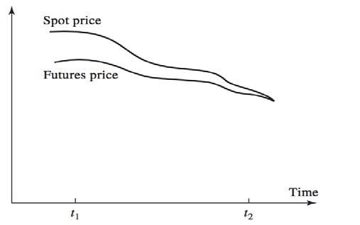
Knowing the spot price, basis reflects the relationship between cash or spot price (S) and futures price (F). 1 1 The today's price in the spot market is the underlying product in futures trading.
It can be over or under as S is higher or lower, respectively than F. It is still generally less volatile than either the cash or futures price. Thus basis is less risky than both spot and futures price. Note that basis (?? 0 ? ?? 0 ) is known by investors on the initiation day, but unknown on the day the hedge will be lifted because ?? 1 ? ?? 1 is a random variable, and the hedger faces strengthened (an increase) or weakened (a decrease) from the time the hedge has been implemented to the F Abstract-Two methods, namely simultaneous bootstrap quantile regression and RiskMetrics, are backtesting and compared to establish which one is a better Value at Risk (VaR) estimate for the United States dollar index returns. Using daily closing prices and the nearby contract settlement prices from 20 November 1985 to 15 February 2017, the results of this empirical research point out that at 5% of the significance level, RiskMetrics with IGARCH (1, 1) underestimates VaR for the next trading day. From the backtest findings, the number of violations in the RiskMetrics method is more than in simultaneous bootstrap quantile regression even after controlling for marginal effects of the index futures returns and volatilities in both spot and futures markets.
3. 2017).
Figure 2 VaR is part of every risk manager's toolbox because it characterizes risk in terms of money while most measures (standard deviation, Sharpe, etc.) show risk as a percentage (Hull and Alan, 1998).
Due to the numerous methods used, which often sound complicated, VaR sounds like a difficult method to evaluate risk. Those models differ in many aspects with common structure summarized in: (1) The portfolio is marked-to-market daily; (2) the distribution of the portfolio returns is estimated, and (3) the VaR is computed (Robert and Simone, 2004). 2
4. i. RiskMetrics method to VaR estimation
Basing on the second aspect, we can classify the VaR methods into two broad categories: factor models, such as RiskMetrics, and portfolio models, such as historical quantiles.
Based on previous studies of Giot and Laurent (2003), Khan (2007), Emilija and Dorié(2011), Askar 2 Three approaches have been used with variations within each. (1) The historical method uses statistical analysis of past losses to determine a loss. (2) The variance method utilizes statistical analysis assuming that returns lie on a bell shape curve based on the average returns and standard deviation. (3) Monte Carlo method involves developing a model and using to predict future investment prices and then using that in statistical analysis to determine the worst-case loss on the investment or portfolio.
Denoting ?? ?? as the daily loss random variable and the information set available at time ??? 1 by ? ?? ?1 , RiskMetrics, a benchmark for measuring risk, assumes that ?? ?? |? ???1 ~??(0, ?? ?? 2 ); where ? t 2 is the conditional variance of ?? ?? , and it evolves according to the model: ? 2 = ?? 2 + (1 ? ?) x 2 ; 0 < ? < 1. By this way, RiskRetrics ignores the fat-tails in the distribution function (Mina and Xiao, 2001). To account volatility clustering of the time series, the RiskMetrics method incorporates an autoregressive moving average process to model the price; and avoid the problems related to the uniformly weighted moving averages by using the exponentially weighted moving average (EWMA) method (Szilárd and Imre, 2000; J. P Morgan, 1996; Pafka, 2001; Tsay 2011).
time when it will be removed (Benhamou, 2005; Hecht, For the reasons above, hedging ambiguously cannot eliminate risk in the underlying asset. To this purpose, investors have to determine and compare the hedge ratio, which is "the ratio of the size of the portfolio taken in futures contracts to the size of the exposure" (Asim, 1993;Hull, 2003). Over the years, methods of calculating the optimal hedge ratio written on a variety of assets (indices, commodities, stocks, and foreign exchange) have been developed: regression method, family GARCH models, which neglect the relationships between returns across quantiles (Sheng-Syan et al., 2003; Bartoszand Zhang, 2010; Mária and Michal, 2016). Thus the risk is still real and will be taken into account, and recent financial disasters have emphasized the need for accurate risk measures. But, as the nature of the risk has changed over time, these methods must adapt to recent experience. Value at Risk is the most recent risk measure (Szilárd and Imre, 2000; Robert and Simon, 2004).
Value at Risk model reports the maximum loss that can be expected by an investor, at a significance level, over an a given trading horizon. Indeed, VaR was developed in the 1990s to provide senior management with a single number that could quickly and easily incorporate information about the risk of a portfolio (Piazza, 2009). Nevertheless, examining different works, its origins lie further back 1990s, traced back as far as around 1922 to capital requirements for the U.S securities firms of the early 20th century. Harry Markowitz (1952) and others developed VaR measure in portfolio theory, where investors have to optimize rewards for a given risk (Glyn Holton, 2002). Nowadays,
5. Global Journal of Management and Business Research
Volume XX Issue I Version I Year 2020 ( ) Deepika (2014), VaR can be calculated through basic GARCH models (GARCH and RiskMetrics), asymmetric models (EGARCH, IGARCH, and GJR-GARCH) and FIGARCH. However, while the sum of parameters in GARCH models is almost close to unity, in the IGARCH model that sum is considered equal to one, which means that the return series is not covariance stationery, and there is a unit root in the GARCH process (Jensen and Lange, 2007). Thus, IGARCH models are unit-root GARCH models. Furthermore, Jensen and Lange argued that "the conditional variance of the GARCH model converges in probability to the true unobserved volatility process even when the model is misspecified, and the IGARCH effect is due to the mathematical structure of the GARCH model and not a property of the true data-generating mechanism."Similar to ARIMA models, in IGARCH
C (2013),?? ?? = ?? ?? ?? ?? , ?? ?? ?? = ?? ?? +?? ?? ?? ?? ????? + (?? ? ?? ?? )?? ?? ????? + ? ?? Equation (2.1)Where {? t } is greater than 0, and 1 > ? 1 > 0.
ii. Simultaneous bootstrap quantile regression method to VaR estimation Quantile regression involves constructing a set of regression curves each for different quantiles of the conditional distribution of the dependent variable. In management (Koenker and Bassett, 1978
?? ?? = (??|?? = ??) = ?? ?? ??(??), 0 < ?? * < 1 Equ ation (2.2)Where ?? (??) is the marginal change in the ?? ??? quantile due to the marginal change in x.
Similarly, if ?? ?? denotes the return of investment at time t, and ?? * denotes a (pre-determined) significance interval, the respective VaR is implicit: Pr[ ?? ?? < ??????|? ?? ?1 = ?? * ; where ? ???1 is the information set available at time?? ? 1. Thus, VaR is the ?? ??? conditional quantile of ?? ?? ; in other words, the one-step-ahead forecast of the ?? ??? quantile of ?? ?? based on the information available up to period?? ? 1. From Equation 2.2, finding a VaR is equivalent to finding the conditional quantile of ?? ?? . Following Christoffersen et al. ( 2001), Engle and Patton (2001), volatility can be treated as a regressor. Since the simultaneous analysis can borrow information across cases and offers tighter inference, the bootstrap method through the "XY-pair method" can be used to know the returns distribution, construct confidence intervals, and approximate coefficients standard errors.
For these reasons, simultaneous quantile regression can be used to compute the U.S. dollar index returns' VaR after the control of the marginal effects of the hedging strategy and returns volatility. This way, differences the research from empirical studies of Robert and Simone (2004), Taylor ( 2008 Then, returns volatility was extracted from the same data using the GARCH (
6. finance, quantile regression can be used to assess risk
While the OLS model estimates the conditional mean of a given ?? = ???? ?? + ?? as ?? (??|?? = ?? = ???? ?? , the quantile estimate however is as specified in equation 2.2 (Huixia, Wang, 2007).
The dataset comes from the global financial portals Investing.com (Madrid, Kingdom of Spain) and Quandl (Toronto, Canada) from 20 November 1985 to 15 February 2017. This period covers the first futures contract on the U.S dollar index as well as the international financial crisis. After the gathering process, data were arranged and analyzed using the R-Software version 3.3.1 (2016-06-21) and Excel. First of all, the daily closing prices of the U.S. dollar index and the nearby contract settlement prices of its futures contract were converted to continuously compounded returns by taking the first difference of the logarithm prices as given in equation (3.1).
Where: ?? ??,?? the continuously compounded daily return at day t; ?? ??,?? the closing and settle prices at day t; ?? ??,????? the closing and settle prices at day ?? ? 1 and ?? the first difference. Furthermore, before the introduction of the Euro to the financial community, the DXY contained ten currencies: the ones that the index includes plus the West German Mark, the French Franc, the Italian Lira, the Dutch Guilder, and the Belgium Franc. Figure 3-1 presents the major currencies included in the index and their corresponded weights. With its 19 countries, the Euro makes up a big chunk of the index (>50%). It is followed by Japanese yen. This position would make sense since Japan has one of the biggest economies in the world. And others with about 25.2%.
7. USDSEK USDCHF
The exchange rate between the Swedish Krona and the U.S. dollar The exchange rate between the Swiss Franc and the U.S. dollar base currency, the index is positive; and negative when it is the quote currency. The price used for the index is the mid-point between the top of the book bid/offer in the component currencies. And at last, the prices of the U.S. dollar index futures contract set by the market reflect the interest rate differentials between the respective currencies and the U.S. dollar (ICE futures U.S., 2015). The U.S. dollar index futures contract began trading on 20 November 1985, on the Financial Instruments Exchange, a part of the New York Board of Trade (NYBOT). Two factors influence the pricing process of contract on this index: (i) the fact that the index is a geometric average, rather than an arithmetic, of the constituent currencies. Therefore, the divergence between the geometric and arithmetic averages depends on both volatilities of the individual currencies and their co-movements; (ii) the FOREX rates in the index (U.S. dollars per foreign exchange rate) are in the denominator, implying that a dollar appreciation leads to a higher index level or a lower level in case of depreciation (Hanan, 1988).
At the end of the day in both spot and futures markets, we can use the price fluctuations between the high and low prices to measure the returns volatility (Gilroy, 2014). Thus, the U.S. dollar index and futures returns volatilities are simply the movements in the first difference of the logarithm of the U.S. dollar index and futures returns. We applied the GARCH (1,1) model to extract both the U.S. dollar index and futures returns volatilities, as written in the following equations. From equations (3.5) and (3.6), the estimation was done in two parts. First, the GARCH (1,1) model was used for the U.S. dollar index returns volatility extraction and then GARCH(1,1) model produces the U.S. dollar index futures return volatility. a) Marginal effects: optimal hedge ratio estimation from quantile regression i. Quantile regression and OLS estimates In table 4-2 results from simultaneous bootstrap quantile regression across four quantiles (25, 50, 75, and 95% quantiles), and the OLS coefficients are summarized. Indeed, all parameters for the U.S. dollar index futures returns, which represent the optimal hedge ratios, are statistically significant (probability = 0) across quantiles. These estimates are not only significant at the confidence level, but are also big than the OLS estimates. The result is consistent with figure 4-1in which estimated optimal hedge ratios across quantiles are above the OLS coefficients, meaning that quantile regression estimated optimal hedge ratios are different from the unique OLS hedge ratio coefficient (at the mean). It implies that the use of OLS, in this case, would underestimate parameters. Therefore the costs of the hedging strategy since quantile regression does not consider only the mean of the U.S. dollar index returns but across quantiles.
8. ?
ii. ANOVA test ------------------------------------------------------------------------------------------------------------------------------------------------- -------------------------------------------------------------------------------------------------------------------------------------------U --------------------------------------------------------------------------------------------------------------------------------------------q50 | ------------------------------------------------------------------------------------------------------------------------------------------- ----------------------------------------------------------------------------------------------------------------------------------------------q75 | --------------------------------------------------------------------------------------------------------------------------------------------- ----------------------------------------------------------------------------------------------------------------------------------------------q95 | ----------------------------------------------------------------------------------------------------------------------------------------------U ----------------------------------------------------------------------------------------------------------------------------------------------OLS | ------------------------------------------------------------------------------------------------------------------------U -------------------------------------------------------------------------------------------------------------------------------------------- - -------------------------------------------------------------------------------------------------------------------------------------------- change across quantiles, and secondly, how the magnitude of the marginal effects in various quantiles differs considerably from the OLS estimators, even in terms of the confidence intervals around each parameter. Moreover, for the OLS method, volatilities' coefficients and the intercept include most zero in their confidence intervals, meaning that these parameters do not have any marginal effects on the U.S. dollar index returns.
However, the intercept differs from zero in lower and higher quantiles; the U.S. dollar index and futures returns volatilities do affect the U.S. dollar index returns across quantiles and depending on the quantile. In some quantiles, the marginal effects are positive and negative elsewhere, implying that both returns volatilities have to be taken into account when estimating VaR. Furthermore, the U.S. dollar index futures return confidence intervals do not include the OLS coefficient, meaning that hedge ratios from quantile regression are all different from the OLS hedge ratio.
9. b) VaR estimation i. VaR from RiskMetrics method
The RiskMetrics method with the Integrated GARCH (1, 1) was conducted to VaR calculation. confidence interval, meaning that Value at Risk increases with the increase of confidence level. At 95 percent of the confidence level, VaR, the maximum negative U.S. dollar index returns, is about 0.0067 dollars one-step-ahead, which means that if the market price goes down, investors who trade the U.S. dollar index will allow to lose up to 0.0067 US$ the following trading day. It seems a small amount for a small investment. However, this loss is highly significant for an investment of millions of dollars. Moreover, the action of removing outliers has a strong effect on the Value at Risk. As showed in table 4-3, VaR has decreased from 0.0067 to 0.0060, that is 11.7%. Meaning that the fat-tail in the dataset distorts the calculation and leads to a pseudo-VaR by overestimating it. For this reason, the VaR without was considered. The significance of this loss was compared through the backtesting process with VaR from quantile regression.
ii. VaR from simultaneous bootstrap quantile regression method From the simultaneous bootstrap quantile regression method, VaR at the 95% quantile is: ?????? ??.???? = ???. ???????? + (??. ?????????????????? * ??. ????????) + (??. ?????????????????? * ??. ????????) + (??. ???????????????? * ???. ????????) ?????? ??.???? = ??. ???????? At 95% of the confidence level, the maximum loss is about 0.0076 U.S dollars for any investment in the U.S. dollar index for the following trading day. It is important to mention that this VaR is the expected loss after controlling for the marginal effects of the U.S. dollar index futures returns and volatilities in both markets. Thus, investors will allow losing money up to 0.0076 dollars.
Results point out that quantile regression VaR removing outliers), a difference of 0.0016 dollars. Note: with the backtesting process, the number of violations is much more in the IGARCH (1,1) than in the quantile regression (904 against 572 trading days) meaning that RiskMetrics 'VaR is allowing more number of negative U.S. dollar index returns. At 5% of the significance level, losses for investors using this method go beyond the VaR 507 times. The violation ratios are 2.3 for the RiskMetrics and 1.4 in quantile regression.
Furthermore, VaR from the RiskMetrics method is lower even using data with outliers (0.0067 and 0.0060 dollars) than the one from simultaneous bootstrap quantile regression (0.0076 dollars), a difference about 0.0016US$ for one unit of US dollar hedged with futures contract over the next day. This difference is understandable because volatilities and futures return marginal effects on the US$ index return are controlled. And globally, these variables are highly significant at 5% of the significance level.
Two methods, namely simultaneous bootstrap quantile regression and RiskMetrics with the IGARCH (1,1),were backtested and compared to establish the better Value at Risk (VaR) estimate for the United States dollar index returns.
Indeed, from the ANOVA test results, all coefficients were significantly different from each other across quantiles. While the OLS intercept and volatilities level, simultaneous bootstrap quantile regression results pointed out that these coefficients were different from zero in the lower and higher quantiles. Marginal effects along the distribution of the U.S dollar index returns were controlled, and hedge ratios across quantiles were also different from the unique OLS hedge ratio, meaning that the cost of the hedging strategy varied across quantiles and was higher than in the OLS method. method did underestimate the maximum loss (VaR). The number of violations (2.3) was much more in the IGARCH (1,1) than in the quantile regression (1.4), which means that the RiskMetrics' VaR allowed more negative or loss U.S. dollar index returns. Furthermore, VaR from the RiskMetrics method was lower (0.0060$) than the one from simultaneous bootstrap quantile regression (0.0076$), about 0.0016US$ of difference for one US$ hedged with futures contract over the next trading day.
Thereby, quantile regression is the best VaR measure because: (1) it allows the hedge ratio calculation, which gives ideas to investors about the value of a position protected through the use of a hedging strategy, (2)the RiskMetrics model ignores the presence of fat-tails in the distribution function, which is a feature of financial data.


| Estimating the United States D ollar Index Returns' Value at Risk: Empirical Evidence from RiskMetrics and | |||
| Simultaneous Bootstrap Quantile Regression Methods | |||
| (actual negative returns). From the Box and Whisker | |||
| outliers detected in the dataset were deleted to eliminate | |||
| their effects for RiskMetrics method since quantile | |||
| regression is robust to outliers (John, 1995; Jason and | |||
| Amy, 2004, Irad, 2005; Hans-Peter et al., 2010, Williams, | |||
| 2016).At the end of all these analyses, two final samples | |||
| were obtained: (1) a sample of 7891 observations | |||
| (representing 99% of the entire dataset) without outliers | |||
| Year 2020 | |||
| Volume XX Issue I Version I | |||
| ( ) | |||
| 042 | 0.036 | Eur JPY BGP CAD SEK | Global Journal of Management and Business Research |
| Model: U.S._dollar_index_returns~ U.S._dollar_index_futures_returns + U.S._dollar_index_returns_volatility + | |
| U.S._dollar_index_futures_returns_volatility | |
| Joint Test of Equality of Slopes: tau in {0.05, 0.1, 0.15, 0.2, 0.25, 0.3, 0.35, 0.4, 0.45, 0.5, 0.55, 0.6, 0.65, 0.7, 0.75, 0.8, | |
| 0.85, 0.9, 0.95} | |
| F value | Pr(>F) |
| 22.192 | < 2.2e-16 *** |
| probability of 0 percent, which is less than 5 percent of the significance level, parameters obtained from | |
| simultaneous quantile regression with 200 replications, with different taus, are high statistically different across | |
| quantiles. The result is consistent with the result in figure 4-1. | |
| U.S._dollar_index_futures_returns | | 0.9537 | 0.0025 | 389.2500 0.000*+ 0.9489 | 0.9585 | |||
| U.S._dollar_index_returns_volatility | -0.1853 | 0.0755 | -2.4500 | 0.014*+ -0.3334 -0.0372 | ||||
| U.S._dollar_index_futures_returns_volatility| 0.3046 | 0.0712 | 4.2800 | 0.000* | 0.1651 | 0.4442 | ||
| Intercept | | Results and Discussion | -0.0003 | 0.0000 | -5.5500 | 0.000*+ -0.0004 -0.0002 | ||
| Year 2020 | |||||||
| Volume XX Issue I Version I | |||||||
| ( ) C | |||||||
| Global Journal of Management and Business Research | |||||||
| Probability | VaR (with outliers) | VaR (without outliers) |
| 0.950 | 0.0067 | 0.0060 |
| 0.990 | 0.0095 | 0.0084 |
| 0.999 | 0.0127 | 0.0112 |
| Year 2020 |
| Volume XX Issue I Version I |
| ( ) |
| Global Journal of Management and Business Research |